As we all know, Excel is an exceptional tool that is packed with myriad features for organizing & analyzing data within the spreadsheet. One such handy feature is the “Freeze Panes.” It allows users to lock the rows or columns in one place so they are visible while scrolling through extensive spreadsheets. However, encountering issues where Excel freeze panes not working can be frustrating. So, let’s delve into this blog to understand this problem and how to fix it effectively.
To repair corrupted Excel file, we recommend this tool:
This software will prevent Excel workbook data such as BI data, financial reports & other analytical information from corruption and data loss. With this software you can rebuild corrupt Excel files and restore every single visual representation & dataset to its original, intact state in 3 easy steps:
- Try Excel File Repair Tool rated Excellent by Softpedia, Softonic & CNET.
- Select the corrupt Excel file (XLS, XLSX) & click Repair to initiate the repair process.
- Preview the repaired files and click Save File to save the files at desired location.
Quick Fixes:
Understanding Freeze Panes In Excel
Excel Freeze Panes option is used to lock row or column headings. So that when you scroll down or view the rest portions of the sheet its top row or first column gets stuck on the screen. In this way, the heading will always appear no matter how you scroll in your worksheet.
Freezing the pane headings is a very helpful feature mainly when you work with the table having information that crosses the columns and rows appearing onscreen.
Where Is Freeze Panes in Excel?
To locate the Freeze Panes feature in the Excel spreadsheet, you have to go to the “View” tab. Now, under the Windows group, you can see the “Freeze Panes” option.
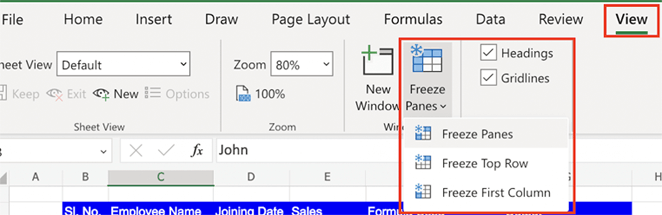
However, if you want to use this feature, select the cells then click on Freeze Panes > Freeze Panes in the view menu. This will immediately lock the selected rows/columns in place to allow maintaining context and reference points for smoother navigation within spreadsheets.
Why Does Freeze Panes Not Work in Excel?
You may encounter this issue when the Freeze Panes option seems grayed out to you or there’s no change in the worksheet after applying this feature. This might happen due to various unexpected reasons, like:
- Either the workbook is protected or corrupted.
- Running an outdated version of the Excel application.
- Incorrect positioning of frozen panes.
- The Advanced Options are restricted in MS Excel Settings.
- When cell editing mode is turned on in the workbook, leading to non-working Freeze Panes.
- Attempting to lock rows/columns in the middle of the spreadsheet.
- The Excel workbook isn’t in the normal preview mode.
How to Fix Excel Freeze Panes Not Working Problem?
To address issues with freeze panes not working in Excel, follow these troubleshooting methods:
Fix 1- Check the Data Size
The very first thing you need to do is to ensure that a dataset is being worked on within the freeze panes feature capacity. If the dataset size is large, consider splitting it into manageable sections for smoother spreadsheet navigation.
Fix 2- Modify Page Layout View
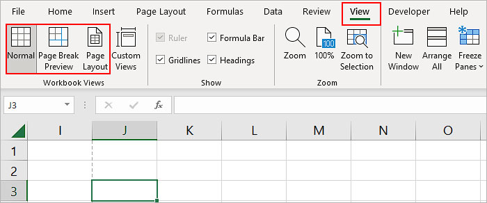
If your Excel workbook is in page layout view then immediately change it to Page Break Preview or normal view. This might be the reason behind facing this problem.
- To do this, tap the View tab from the Excel menu.
- After that, from the Workbook Views group, choose any option other than the page layout view. Like normal, page break preview, or custom views.
Fix 3- Exit from Cell Editing Mode
Using worksheets in a cell editing mode can sometimes impact the datasets, disable certain features, and cause various issues including freeze panes Excel not working. In such a case, disabling the cell editing mode can come in handy. To do so, press the Enter or ESC key. Now you can check if the issue is resolved or not. If not, move to the next solution.
Fix 4- Unprotect The Worksheet
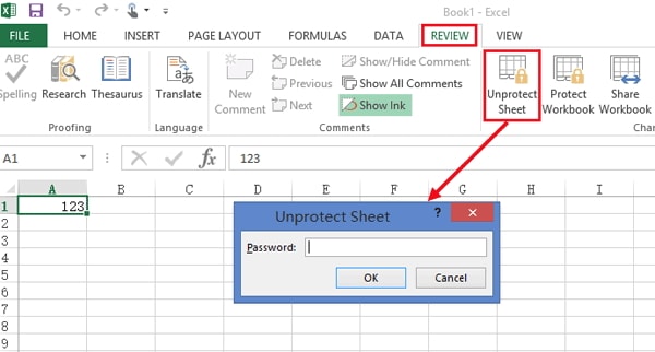
If the Windows option for Workbook Protection is enabled, it will make your Freeze Panes feature not work. Well, this Windows option seems permanently disabled in Excel 2016 and 2013. To enable the Freeze Panes option again, you need to unprotect your Excel workbook:
- Tap to the Review tab from the Excel ribbon.
- Click on the Unprotect Sheet.
- In the opened window type the password, and then click OK.
Like the Page Layout view, the Protect Workbook doesn’t undo the freeze worksheet panes. It only prevents you from freezing and unfreezing the worksheet pane until and unless your workbook is protected.
Fix 5- Checking the Excel Version to Fix Excel Freeze Panes Not Working Issue
As already mentioned in the causes section, if you are running an outdated version of an Excel application, it can hinder the freeze panes feature. All you need to do is check and ensure that the Excel version being used supports the freeze panes and is updated. If it is not updated, Click Here to check and install the latest version and fix compatibility issues.
Fix 6- Unfreeze the Worksheet Pane
Another method through which you can escape freeze panes Excel not working is by unfreezing the worksheet pane. Follow the below simple steps to unlock all columns and rows of your Excel sheet.
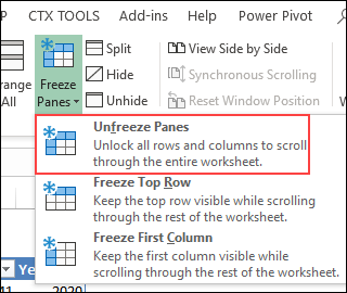
- At first tap to the View tab and now from the Window group, choose the Freeze Panes arrow sign.
- From the drop-down menu choose the “Unfreeze Panes”.
Fix 7- Fix the Problem by Disabling Options in a Data Tab
If you have enabled any customized features under a Data tab in your worksheet like Sorting, Filter, Group, etc, leading to unforeseen hitches with the freeze panes feature. Consider verifying & disabling these features in your sheet. Follow the below instructions carefully to do this:
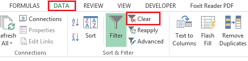
- Open the faulty Excel file >> go to “Data” tab.
- Then, check and disable features like Sort, Filter, Subtotal, and Group.
Also Read: Resolve Excel Flash Fill Not Working Issue Easily!
Fix 8- Use The Table Instead Of Freeze Top Row
As an alternative to the Freeze Top Row option, you can format your data just like a table. As in the table, Excel replaces the letters of the column with top rows content when you scroll down.
Here’s what you need to do:
- Go to the Home tab and now from the style group choose the Format as Table.
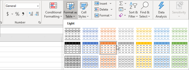
So when scroll down in your Excel sheet, note that your column number will attain the position of header titles.
It will appear in that way as you scroll down in the worksheet.

(If you choose or activate any cell across from the table, then the headers will automatically get disappear and column letters will start reappearing.)
Fix 9- Repair Corrupted Excel Workbook
File corruption is the foremost reason for triggering various problems or errors in Excel. So, if you are suspicious that freeze panes greyed out or freeze panes not showing in Excel due to workbook corruption, you can go for the Excel’s Open and Repair utility to repair your file.
Follow these instructions to learn how to use this tool:
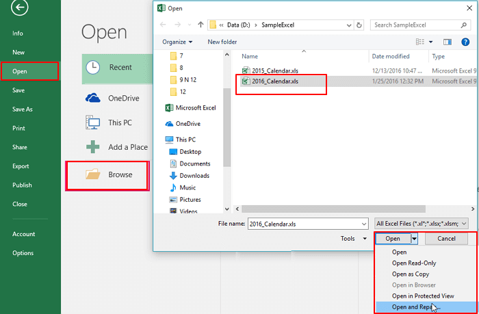
- Open Excel application >> click File >> Open >> Browse.
- Select the corrupted file in which you’re facing the problem.
- Click an arrow next to an Open option >> then Open and Repair.
- After that, click Repair button to regain as much data as possible.

- Finally, click Close after completion of the repair process.
If the Open and Repair utility won’t work, in that case, you need to use the MS Excel Repair Tool to fix the corruption in your Excel workbook.
Some Highlighting features of this Excel repair tool:
- It is a unique tool that repairs multiple corrupted Excel files at one time.
- It is capable of recovering charts, cell comments, worksheet properties, and other data without modifying the original format.
- This is the best repair utility to repair all sorts of damages, corruption, and errors in the Excel file.
Fix 10- Try Other Workarounds
Apart from the above solutions, you can try some other fixes like:
Related FAQs:
What Happens When the Freeze Panes?
Freezing panes in Excel helps to keep certain rows or columns visible when scrolling across the spreadsheet.
Can I Freeze Row and Column at The Same Time?
Yes, Excel’s Freeze Panes allows you to freeze both rows & columns at once, providing flexibility in data navigation.
What Is the Shortcut Key to Freeze Rows and Columns in Excel?
Alt+W+F+F is the keyboard shortcut to freeze rows and columns in Microsoft Excel.
What Should I Do If Freeze Panes Cause My Worksheet to Become Unresponsive?
After applying the freeze panes feature, if it impacts worksheet performance, you should try to reduce the number of frozen rows or columns.
Why Can't I Freeze Both Column and Row in Excel?
It might possible that your workbook is protected/corrupted or you are attempting to lock rows/columns in the middle of the Excel spreadsheet.
How Do I Freeze Multiple Non Consecutive Rows In Excel?
Well, it is not possible to freeze non consecutive rows in Excel. Freezing is possible only for one column or row.
Wrap Up
Undoubtedly freezing Panes is a fantastic option to quickly overview when the dataset is huge. Now you don’t need to bother with these hidden columns and rows problem which arises due to freeze panes not working in Excel issue.
All the listed solutions in this blog are tried and tested, so they will surely resolve your problem.
If you encounter any problems meanwhile performing these fixes or get into some other issues, do share your problems with us through our social media FB and Twitter Pages.

Priyanka Sahu
Priyanka is a content marketing expert. She writes tech blogs and has expertise in MS Office, Excel, and other tech subjects. Her distinctive art of presenting tech information in the easy-to-understand language is very impressive. When not writing, she loves unplanned travels.