Microsoft Excel is very popular and best application for managing, organizing and arranging crucial data.
This application is used in countless ways and this is the reason numbers of features are packed inside this Microsoft’s popular application.
This doesn’t matter whether you are a casual user or an Excel expert, it is important to know everything in it so that you can easily use this complex application.
Here in this article, we are describing – easy tips n tricks that will make you master Microsoft Excel:
Included Excel Tips and Tricks:
Tips and Tricks to Master Microsoft Excel
1. Click once to Select All

Many of us know that we can select the entire excel sheet by using the Ctrl + A shortcut but I guess few of us know that simply clicking once on the corner button will select the entire data in less than a second.
2. Open Multiple Excel Files at Once
While working on multiple excel files, you need to open files one by one, this is quite difficult to handle but here we will describe a handy way to open them all with one click.
All you need to do is to select the files you like to open and press Enter key, all selected files will open altogether.
3. Create a New Shortcut Menu
Using shortcuts makes the work easy. In Excel we are having three shortcuts in the top menu – Save, Undo Typing and Repeat Typing.
But if you want to utilize more shortcuts like Copy and Cut, you can set them up:
Here know how:
Go to File > Options > Quick Access Toolbar > Add Cut and Copy from the left column to the right and save it.
Now you can see two more shortcuts added to the top menu and make the work easy for you.
This is really very helpful to organize the Excel crucial data easily and become an Excel expert.
Know More MS Excel TRICKS.
4. Add More Than One New Row or Column
Well, I think most of the Excel user must know that by selecting a row or column we can add a new one via Insert drop-down under Home.
However, here is an easy way to do so.
Drag and select rows or columns > right click the highlighted rows or columns > select Insert from the drop down menu.
Now new rows will be inserted above the row or to the left of the column you first selected.
NEXT…
5. Apply Diagonal Borders
If you got a table that requires both row and columns headers in the same cell then make use of the diagonal borders.
Click More Borders at the bottom of the borders drop-down menu (on the Home tab of the ribbon) and diagonal buttons are by the box corners.
Click it and save.
This makes the work easily understandable and presentable in your excel sheet.
Additional Reading:
6. Turn Columns into Rows

If you have data in columns that should be in rows or the other way then here we have tips to do so without losing anything.
Just, copy the original block of the cell > right click on the destination cell > click Paste Special > Transpose.
7. Hide Individual Cells
Excel has a master trick of hiding cells. This is one of the best Excel tips and tricks
All you need to do is to select the cell that you want to hide and right click >select Format Cells and then set the format as Custom under the Number tab and Enter;;; (three semicolons) as the format.
Now the cell content disappears but they are still present there and can be used in formulas.
This is really amazing Excel tips and tricks
8) Freeze Row and Column Headings
This is the simple but useful trick to becoming an Excel expert.
Freeze the row and column headings so they are always viewable when you scroll around.
To do so, LOOK
Place the cursor in the top-left cell where the actual data starts and go to VIEW menu and simply select Freeze Panes and Freeze Panes.
Now the heading is viewable where ever you scroll.
9. Quickly Move and Copy Data in Cells
If you want to move one column of data in a spreadsheet then the easy and fast way is to select it and move the pointer to the border after it turns to a crossed arrow icon then drag to move the column freely.
But if you want to copy the data, .then press the Ctrl button before dragging to move the new column will copy all the selected data.
10. Delete Blank Cells Fast
Some of the default data will be blank for various reasons.
So if you need to delete these to maintain accuracy, particularly while calculating the average value.
The easy way is to filter out entire blank cells and delete them with one click.
Choose the column you want to filter and go to Data > Filter after the downward button shows, undo Select All and then pick the last Blanks option.
The entire blank cell will show immediately.
Now go to Home and click Delete directly, all will be removed clicking once.
11. Use Flash Fill to Save Time

Flash fill makes the work easy, so if you are reformatting data in adjacent columns, then this is very helpful.
It recognizes the patterns and fills the rest of the details for you.
Just give excel a few examples at the top and you will see the suggestions in gray, hit Enter to accept.
12. Add Comments to Your Formulas
Add space and +N (“your comment here”) to leave comments by your formulas for your own reference or to help other people understand your spreadsheet.
Comments don’t appear in the cell but show up in the Formula bar and they are searchable as well.
13. Quickly Add Up Figures
It is likely that you are doing a lot of addition to Excel, but here you don’t need to type out SUM formulas.
Just highlight the cell at the end of the row or the bottom of the column you want to add and then hit Alt+= ( equals) or Cmd+Shift+T on a Mac
14. Rotate Heading Text
If you need to add headers to very narrow columns, then rotate the text to fit.
Go to Home tab and click the Orientation button and make your choice.
The button is placed alongside the other text formatting options. This is another effective Microsoft Excel tips and tricks.
15. Add Decimal Points Automatically
Here we will tell you the trick to add decimal automatically. There is no need to waste time manually inserting the decimal points.
Click File > Options > Advanced and the option is near the top.
Here you will find various useful settings on this page, covering program behavior, number formats and much more.
Find more interesting Excel tips and tricks.
Look…
16. Add Your Own Graphics to Charts
While making charts graphics you don’t need to settle for the colored blocks that by default Excel offers.
All you need to double-click on a bar and then click paint bucket to change the fill options.
You can also switch to gradients, a pattern, or load in an image file from disk.
17. Save Charts As Templates
This is another handy chart related trick to make yourself the master of Excel.
When you found a combination of layout and colors that are really important, save it as a template, so that you can utilize it again.
Right-click on any chart created and you will see the Save as Template option.
18. Add the Calculator (or else) to Quick Access
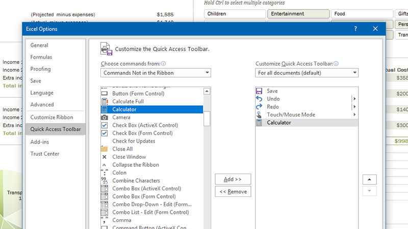
In your excel file, you can add shortcuts like calculator, Windows Camera or Ink apps or the zoom controls.
This makes your work easy in Excel document.
You can do this by opening the Quick Access Toolbar (to the right of the save and undo commands on the title bar) > select More Commands > and add the shortcut to the menu whatever you like.
19. Apply Some Conditional Formatting
In Excel, you can add Conditional formatting this can add some pop to the sheets and helps you pick out data easily.
It is simple to use.
Select the data that is needed to be formatted > click Conditional Formatting (in Home) > and build your rules accordingly from the drop-down options.
20. You can Draw Equations
This feature is available in Excel 2016 (useful if you are having a touchscreen PC).
To draw equations you need to go to the Insert tab on the ribbon menu and select Equation and Ink Equation.
And after that, you can sketch in the yellow box.
21. Fast Navigation with Ctrl + Arrow Button
Here is a trick to make fast navigation in Excel many of us know that when we click Ctrl+ any arrow button on the keyboard, you can jump to the edge of the sheet in different directions.
But if you want to jump to the bottom line of the data, just click Ctrl+ downward button and easily go to the last cell.
22. Input Values Starting with 0

This is very important for the regular Excel users.
When any input value starts with zero, Excel by default deletes the ZERO.
So rather than reset the Format Cells, this problem is easily solved by adding a single quote mark ahead of the first zero.
23. Rename Sheet Using Double Click
There are numerous ways for renaming sheets and many users will right click for selecting Rename, this is a process.
The easiest and fast way to rename is to click twice and rename it directly without wasting time.
This is not the end.
Check out more interesting EXCEL TIPS.
24. Compose Text with &
The & symbol is very necessary to compose any text freely.
For example: below you are having four columns with different texts, but if you want to compose them to one value in one cell.
Then first locate the cell that is to display the composed result, utilize the formation with & and hit Enter.
The entire text in cell, A2, B2, C2 and D2 will be composed together in the F2 cell.
25. Transform the Case of Text
In this article, I have tried by best to avoid complication formulation.
But there are yet some simple and handy formulations like UPPER, LOWER and PROPER that can transform texts for different purposes.
Upper will capitalize entire characters; LOWER changes the text to lower case and PROPER only capitalizes the first character of a word.
Really amazing…
26. Speed up Entering Complicated Terms with AutoCorrect
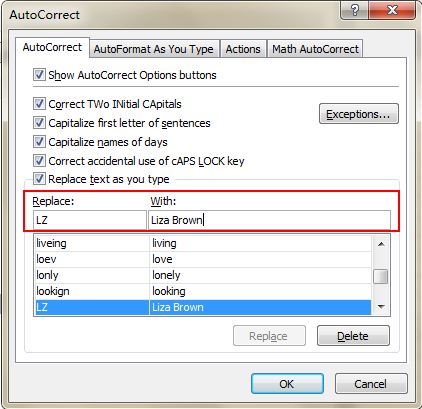
While working in an Excel file if you need to repeat same value and it is quite complicated to enter it.
Then here know how to do it easily by using the AutoCorrect function.
Doing this will replace the text with the correct text.
For example: Take any name like Amy Jackson, and replace it AJ, and after that every time you enter AJ, it will autocorrect to Amy Jackson.
This is really an interesting and useful Excel trick.
To do so:
Go to File > Options > Proofing > AutoCorrect Options and enter Replace text with correct text in the red rectangular area,
27. Generate a Unique Value in a Column
Many of the Excel users are well aware of the key function of Filter but few of them utilize the Advanced Filter.
This helps the users to repeatedly apply when you need to filter a unique value from data in a column.
Follow the Process:
- Click to select the column and go to Data > Advanced > a pop-up window appears
- Next click Copy to another location, which is in the second rectangular area
- And after that specify the target location by entering the value or clicking the area choosing button.
- Now the unique age is generated from column C and will appear in Column E.
- You also need to select Unique records in the pop-up
- Click OK
Now, the unique value showing in column E could be a contrast of the original data in C.
This is the reason why it is recommended to copy another location.
28. Input Restriction with Data Validation Function
To retain the validity of data, in some cases it is required to restrict the input value.
And offer some tips for further steps.
For Example, Age in the excel sheet should be in whole numbers and the participant in the survey should be between 18 and 60 years old.
So to make sure, data outside of this age range should not be entered.
Go to Data > Data Validation > Setting, input the circumstances and modify to Input Message to give prompts. Like (Please input age in the whole number and should in the range from 18 to 60).
Users will automatically get this prompt while hanging the pointer in this area as well as get a warning message if given information is unqualified.
29: Bring Selection into View

This Excel tips will help you to easily recognize the selection area.
Suppose if have selected some areas of cells and scrolled away and now you are unable to see it
… then, in this case, hit Ctrl + Backspace key this will brings that selection into view.
And if you hit Shift + Backspace it will bring the selection into view but reduces the selection to the active cell.
30. Learn Excel’s Best Shortcut Keys
Well, this is the last tips and tricks of our article and this is very helpful for the Microsoft Excel users to fix the error.
You should learn some shortcut keys to increase your productivity in Excel.
Here we have included some shortcut keys that are useful for regular work.
- Ctrl +[Down|Up Arrow Key]: This is used to move to the top or bottom cell of the current column and using Ctrl with Left|Right Arrow key, moves to the cell furthermost left or right in the current row
- Shift + Ctrl + Down/Up Arrow: It will select entire cells above or below the current cell
- Ctrl+ Home: Go to cell A1
- Ctrl+End: To go to the last cell that contains data
- Alt+F1: It will create a chart based on the selected data set.
- Ctrl+Shift+L: This will activate an auto filter to the data table
- Alt+Down Arrow: For opening the drop-down menu of the auto filter. To use this shortcut:
- Alt+D+S: For sorting the set data
- Ctrl+O: Open a new workbook
- Ctrl+N: Create a new workbook
- F4: To select the range and press F4 key, this will change the reference to absolute, mixed and relative.
End Note:
Hope after reading this article, you get the ample information about the Excel features.
You can make use of the tips and tricks to increase your productivity in Excel and get all your work done quickly.
So start using the features included in this article and become an Excel expert now.

Priyanka Sahu
Priyanka is a content marketing expert. She writes tech blogs and has expertise in MS Office, Excel, and other tech subjects. Her distinctive art of presenting tech information in the easy-to-understand language is very impressive. When not writing, she loves unplanned travels.