Unlocking the Secrets to Filter Out Excel Data to Save Time and Effort

As we all know, filters are a handy tool in Microsoft Excel for managing & analyzing data in a spreadsheet. Whether you are dealing with large or small datasets, filters can save your valuable time & improve the data analysis efficiency. Many Excel users don’t know the best of using it and carrying out various functions easily in Excel. In this post, I will describe the amazing thing about Excel filters and how you can filter out Excel data to save time.

Let’s get started…

Understanding Data Filtering

In Excel, data filtering is a method that allows you to display exact data from the larger dataset, making it easier to work with and analyze. This feature instantly sorts & displays the data you need, while the rest of the information fades into the background.

Types of Filters in Excel

There are various types of Excel filters that you can use to manipulate & analyze data. Here I have listed the common types of filters, let’s take a look:

1. Text Filters: The text filters allow you to filter the data in text columns.
2. Number Filters: The number filters allow you to filter the info in numeric columns.
3. AutoFilter: This filter allows you to filter out the data in a column based on exact criteria.
4. Date Filters: You can use this filter based on specific date criteria, like dates that are after, before, between, or equal to a certain date.
5. Filter by Color/Cell Color: Filter by Color allows you to filter data based on the cell background or font color.
6. Filter by Condition: It allows you to set the custom filtering conditions based on the formulas.
7. Top 10 Filter: It allows you to show the top or bottom “N” items from a dataset, like the top 10 sales figures or the bottom 5 performers.
8. Filter by Selection: You can filter the data based on value selected in an exact cell.
9. Advanced Filters: This filter offers complex filtering capabilities, as well as the ability to filter data based on multiple criteria and extract filtered data to a new location in the worksheet.
10. PivotTable Filters: Under PivotTable, you can apply the filters to columns, rows, values, etc. in the Excel table to drilldown into certain data subsets.

How to Filter Out Excel Data to Save Time?

Follow the below ways to filter out Excel data to save time:

1. Filter Out Data by Number Filters or Text Filters 

If you want to filter out a range of data whether it is texts or numbers in the columns/rows, follow the below steps:

• Select the range of cells.
• Choose Data then Filter.
• Next, select a column header arrow .
• Choose either Text Filters or Number Filters.
• Select the comparison, such as Between.

• Now, enter the criteria of the filter and click on OK.

2. Enter in the Search Bar

This way is simple and highly effective. Well if you are utilizing Excel 2010 and later version then in your filter drop-down menu search bar is available.

And, then check the below data table where you need to filter results. You can filter it by names for example “Sam”.

Here follow the steps:

• First, add filters to your data.
• Then, open the filter drop down > click on the search bar.
• In the search bar, type the name that you want to filter Eg. “Sam”

• As you do that, this will filter the entire values where word “Sam” is presented.
• Lastly, click OK.

The best thing about the result is it is highly active and gives the results right at the time when you type your search.

#Bonus Tip: if you need to search for a date make use of the little drop-down from the search bar right side to choose if you need to search for a year, month, or date.

3. Use Date Filters

Date Filters are the smartest tip to filter out dates easily. There are a lot of options that you can utilize to filter dates and when it comes to date Excel is very good.

In the below list,  you can utilize them, they are highly useful.

• Year to Date: This is highly useful if you want to filter the entire data from the year starting to till date.
• All Dates in a Period: This helps you to filter entire dates within a particular month or quarter.

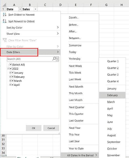
There are a total of more than 21 custom filter options for dates. And, if you need to filter custom data, you can utilize a custom filter.

You May Also Read: Ways to Delete Highlighted Cells in Excel Instantly

4. Filter By Color

Filter by color is a highly creative technique to filter values. When some cells in the worksheet are highlighted with color, they can be easily filtered out.

The highlighted color is extremely easy to filter out names, data, or some errors that you want to filter all those cells.

Follow the steps to do so:

• First, to your data apply a filter.
• Then open the filter drop-down.
• And go to Filter by colour > choose the colour for which you want to filter.

• Since as you click on the colour, this will filter the entire cells with the red colour

The best thing about the filter option is user can filter the cells where there is no colour.

5. Filter by Condition

This filter option works best with more than one situation. You can utilize Filter by Condition when requiring filter values if one of two given circumstances is met or both the conditions are met, then you can do this by utilizing OR in Excel filters.

For example: In your entire company data, you need to filter only for the people whose name is “Sam” and “Sammy”. This will help you to filter out Excel data to save time easily.

Know here follow the steps to do so:

• First, add filters to your data.
• Then for the column where you need to filter data > open filter drop down.
• Next, go to > Text Filters > Custom Filters.

• A window appears to select filters options.
• From this window > choose “contains” from both the drop downs.
• Next, in the input bar type “Sam” and in second input bar enter “Sammy”.
• From the options button > choose “Or”.

• And lastly, click OK.

Now, from the entire cell where you are having “Sam” and “Sammy” are filtered easily.

#Bonus Tip: Well, if you want to filter values based on two conditions for instance: if you want to filter cells where you are having both “Sam” & “Sammy” in a single cell, make use of AND, instead of using OR.

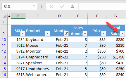
6. Filter Top 10 Values

Here in this tip, you can filter the top 10 values easily. If you have a large dataset and from the data, you need to check the top 10 values, then do this easily in a few clicks.

Follow the steps to do so:

• First, apply filters.
• Then from the column where you want to filter > open filter drop down.
• Go to > Number or Value Filters > Top 10

• This will open a pop-up window. And from that window, choose the following things.
  • Top or Bottom Values: To choose top or bottom values to filter.
  • Number of Values: To identify the numbers of values you need to filter.
  • Type of Filter: This is an elegant option, where you can select the way you need to filter values.

• As the preference is selected by you, click OK.

Since you click OK, the entire values in top 10 will be filtered

7. Filter Above/Below Average Values

This is a useful tip for checking the data insight. You can use this if you want to filter values that are above average. Then here know the easy trick to do it easily by applying Excel filters.

Follow the steps to do so:

• First, on the column apply filters > where you have values.
• Then, open filter drop-down > go to “Number Filters” > click on “Above Average”.

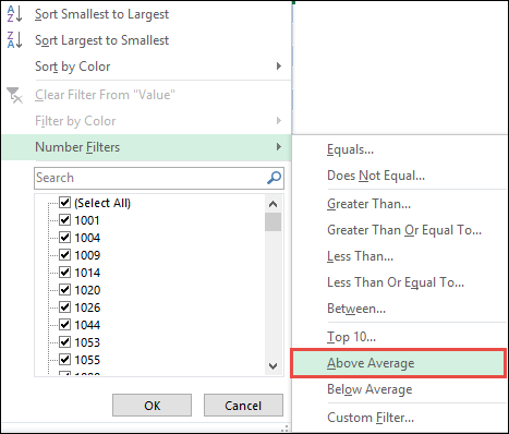
• As you do this it will filter the entire values which are above average.

Well, you can make use of the same method to filter values that are below average. Simply click on “Below Average” in place of Above Average.

Also Read: Excel if Blank Then Skip to Next Cell (Full Guide)

8. Utilize a Wildcard Character

Wildcard characters are about partly matching and finding the text. And this can now be used for filtering values.

For example: if you want to select the names that start with letter “H”, then you can do this easily in the name list.

Here know how:

• To your data apply filters.
• Open filter drops down.
• Then, in the search bar type “H*”.
• As you type the text, this will quickly filter the entire names that start with the “H”

• And click OK

This method is utilized with the custom filter option.

9. Filter Values in Pivot Tables

The best way to filter values in Pivot Tables is by utilizing slicer. With the help of this, you can link multiple pivot tables to one filter with a slicer.

Follow the steps:

• Create a pivot table > click on any of the cells in it.
• Then, go to Analyze Tab > Filter > “Slicer”.

• This will quickly give you a pop-up window to choose the field you want to sue in the slicer.

• Then, click OK.

Now, utilize the slicer to filter entire values in the pivot table.

The best thing about the slicer is that it can check any time, how many values you have to use as a filter.

How to Filter Out Excel Data in A Table?

When you enter data in a table of your Excel spreadsheet, the program will automatically include the filter controls on columns if they’ve headers. In order to filter through these controls, you have to follow the below instructions:

• Select an arrow of the column header for the column you need to filter.

• Then, uncheck the ‘Select All’ >> select boxes that you need to display.

• Choose OK.

Now, the column header arrow will change to the Filter icon. choose this icon in order to change the filter.

Don’t Miss: Most Underrated Excel Functions You Must Try

Related FAQs:

Are These Methods Suitable for Beginners?

Absolutely, the methods explained above in this post are beginner-friendly.

Can I Apply Multiple Filters in Excel Simultaneously?

Yes, of course, you can use multiple filters in Excel to refine your spreadsheet data further.

Are There Keyboard Shortcuts for Excel Filters?

Yes, there are keyboard shortcuts that Excel users can use to expedite the filtering process.

Do Excel Filters Work in Older Excel Versions?

The answer to this question is No. The filters may not work properly in the older versions of Microsoft Excel.

Can I Undo a Filter in Excel?

Yes, you can undo a filter in Excel by clicking the filter icon again. This will return your data to its original state.

Can I Enhance the Performance of Excel When Using Filters with Large Datasets?

Not all the time, but sometimes you can enhance the performance of Excel when using filters with large datasets.

How Can I Remove a Filter in Excel?

You can remove a filter in Excel by clicking on the Filter icon in the column header and then selecting the ‘Clear Filter.’

Final Thoughts

Effective data filtering is an appreciated skill that can improve your productivity & decision-making capabilities. With the advanced practices outlined in this blog, you can filter out data in MS Excel to save time & effort when working with spreadsheets.

I hope you liked this guide.