ISERROR Function in Excel Secrets – Fix Excel Formulas in Seconds (2025 Update)

In Microsoft Excel, various formulas and functions are used to perform simple and complex calculations. One such function stands out for its error-detection capabilities: “ISERROR.” It helps to detect a specific cell that contains an error value, paving the way for a healthy & error-free spreadsheet. Well, in this post, I will provide a brief overview of this function & explore how to use ISERROR function in Excel for easy calculations.

What Is the ISERROR Function in Excel?

The Excel ISERROR function is a part of the Information functions category. It is used in conjunction with the IF function to detect a potential formula mistake & display other formulas or text strings as messages or blanks. If an error is detected, it can also be utilized with the IF function to show a custom message or conduct some other calculation.

If the provided value represents an error, the function will return TRUE; otherwise, it will return FALSE. In simple words, ISERROR can enhance the report’s appearance and spare you from embarrassment.

Syntax of ISERROR Function

Below you can the syntax of this function:

ISERROR function in Excel applies the argument as shown below:

Value: This is the targeted cell that you need to test. It is mostly provided as an address of the cell.

What Errors Detect by ISERROR Function?

The ISERROR function catches all sorts of errors, including #NAME?, #NUM!, #VALUE!, #DIV/0!, #N/A,  #REF!, #CALC!, #SPILL!, or #NULL.

Also Read: How to Use IFERROR In Excel? – IFERROR Insights & Pro Tips

How To Use ISERROR Excel Function?

Consider the following scenarios to better understand the ISERROR Excel function:

Example 1:

Let’s look at the function’s output when we submit the following information:

Example 2:

We may utilize the ISERROR function wrapped in the SUMPRODUCT function to count the number of cells with errors.

Let’s say we’re given the following information:

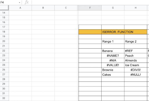
Using the formula =SUMPRODUCT(–ISERROR(G22:CH27)), we can get the count of cells with an error, as shown below.

In the above formula:

The SUMPRODUCT function accepted one or more arrays and calculated the sum of the products of corresponding numbers.

ISERROR now evaluates each of the cells in the given range. The result will be TRUE,FALSE,FALSE,FALSE,TRUE,TRUE,FALSE,TRUE,TRUE,TRUE,FALSE,FALSE.

As we used double unary, the results TRUE/FALSE were transformed to 0 and 1. It made the results look like {0,1,1,1,0,0,1,0,0,0,1,1}.

SUMPRODUCT now sums the items in the given array and returns the total, which, in the example, is the number 6.

As an alternative, the SUM function can be used. The formula to use will be =SUM(–ISERROR(range)). Remember to put the formula in an array. For the array, we need to press Control + Shift + Enter instead of just Enter.

Example 3:

Here in this case we will see for instance if we wish to provide a custom message, for example, instead of getting #DIV/0 error, we want the value to be 0. We can use the formula =IF(ISERROR(A4/B4),0, A4/B4) instead of A4/B4.

Suppose we are given the following data:

Instead of TRUE, if we want to enter the value 0, the formula to use will become=IF(ISERROR(B6),0,B6) and not B6, as shown below:

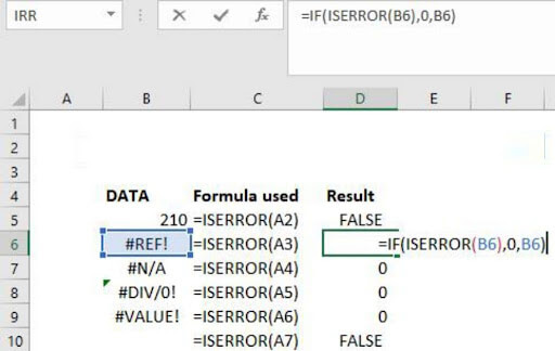
We get the result below as shown:

Method for Manually Replacing ERROR Values

However, we may use the ISERROR, formula to replace the error; there is one manual approach for doing so: the discovered and replace method.

1. After applying the formula, copy and paste only the values.
2. To open the replace box, press Ctrl + H and type the error value (#N/A, #DIV/0!, etc.). Make a note of the sort of error you’d like to replace.
3. Substitute “Data Not Found” for the replace with values.
4. Select Replace All from the drop-down menu.

All of the previously specified error values would be replaced with Data Not Found as a result of this.

Note: If you’ve applied a filter, the visible cells-only technique should be used to replace it.

Best Practices for ISERROR Function

1. Always combine ISERROR with IF when you need custom messages.
2. Use it in complex formulas to detect hidden calculation issues.
3. Avoid overusing it, as it can slow down large workbooks.
4. Consider switching to IFERROR for simpler error management.

Don’t Miss– Everything You Need to Know About Excel Matrix Functions

Related FAQs:

What Is the Difference Between Iserror and Iferror?

ISERROR functions checks if the value is an error & returns TRUE or FALSE, whereas IFERROR function returns the specified value if a first argument is an error,

Can ISERROR Only Detect Numeric Errors?

No, ISERROR can detect various types of errors, including those associated to text & formulas.

Why Do We Use the Iserror Function in Excel?

The IsError function in Microsoft Excel is used to control if a numeric expression represents an error.

Does Using ISERROR Affect Excel's Performance?

No, Excel ISERROR is not affecting Excel’s performance as it is lightweight function & has a slight impact on program’s performance.

Time to Wrap Up

After going through this entire post, you must have gotten complete information regarding the ISERROR function in Excel. This may enhance your numerical reports by rejecting all types of mistakes. Consequently, follow the step by step on how to use this function to enhance the report’s appearance.

Additionally, if you have any queries related to this topic, then ask on our official Facebook & Twitter pages.