Unlock Your Potential: Excel If Blank Then Skip to Next Cell Revealed!

Blank cells within MS Excel refer to cells that do not contain any data. It happens due to numerous reasons like incomplete entries, data extraction issues, or intentional gaps in data sets. Sometimes, the blank cells in a spreadsheet can affect calculations, sorting, and filtering processes, leading to errors & data inconsistencies. Well, in this blog, I will mention some easy solutions for Excel if blank then skip to next cell. So, let’s check out this blog without skipping any section.

What Happens If A Cell Is Empty Then Return Value?

If a cell is empty within the Excel worksheet and you are performing the ISBLANK function, it will return “TRUE.” But if a cell holds an empty string (“”), then the ISBLANK function will return “FALSE.” In such a case, you will have to skip/move to the next cell if a cell is blank by applying the effective methods mentioned in the next section.

Ways For Excel If Blank Then Skip to Next Cell

In this section, I will show you how to skip the blank cells using different formulas & retrieve the values from next cell. Here, we will work on the list of IDs, Products, & their equivalent Sales values where some cells are blank in the Product & Product ID column.

Now, let’s follow the below step-by-step methods to move to next cell in Excel.

Way 1- Use IFS Function

The very first function that you can use to go to the next cell is IFS function. The IFS function in MS Excel displays whether one or more conditions are observed & returns the value.

So, let’s use IFS function and follow the below steps to skip the empty cells of a Product ID column & move to Product column.

Step 1- Initially, enter the below formula in a E4 cell.

In this formula, B4 is a Product ID & C4 is a corresponding name of the Product.

Step 2- After that, hit the ENTER key & drag down a Fill Handle.

At last, you’ll get the products list without IDs of Products in a List column.

Also Read: Fix VLookup Invalid Cell Reference Error In Excel

Way 2- Use IF & ISBLANK Functions in Excel

Here, you have to use the combination of two Excel Functions, one is IF, and another is ISBLANK. This will help you to combine the product name which doesn’t have the equivalent Product IDs and will give you the result.

So, follow the below steps for Excel if blank then skip to next cell VBA:

• First of all, enter the below formula in E4

In the above formula, B4 is a Product ID & C4 is a corresponding name of the Product. In case, if B4 cell is blank, it displays the name of the product ‘Apple’, otherwise empty.

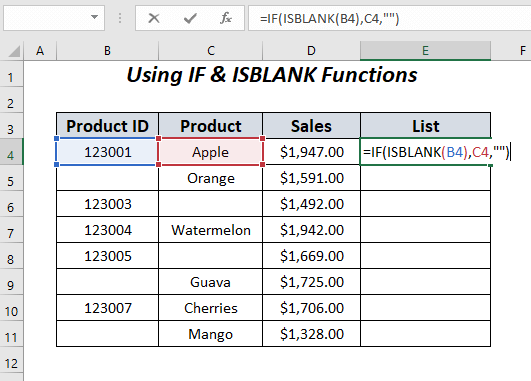
• Now, hit the ENTER key & drag down a FillHandle.

If this method doesn’t work, proceed to the next one.

Way 3- Use the IF Function

The IF is a useful function in MS Excel that allows you to make the logical comparisons between two values. On the other hand, we can say, IF is a premade Excel function, which returns the values based on True or False state.

So, here I will show you how to use this function to make a list of the product name which don’t have the equivalent Product IDs and will give you an accurate result.

Follow the below steps for Excel if blank then move to the next cell:

Step 1- Initially, enter the below formula in an E4 cell.

In the above formula, B4 is a Product ID & C4 is a corresponding name of the Product. In case, if B4 cell is blank, it displays the name of the product ‘Apple’, otherwise an empty.

Step 2- Hit ENTER & drag down a Fill Handle.

In the end, you will get the following results in your list column.

Also Read: Quick Ways to Remove Blank Rows in Excel

Way 4- Skip to Next Cell If It Is Blank in Excel by Using IF & XLOOKUP Functions

Now, I will recommend you use the combination of two Excel functions, one is the IF & another is XLOOKUP. Using these Excel functions simultaneously will assist you to skip to next cell if it is blank.

Here is how to skip blank cells in Excel using IF & XLOOKUP Functions:

• Initially, keep the first cell of a List column as the Blank.

• Then, put the below formula in D5 cell.

• After this, you have to hit ENTER key & and drag down a FillHandle.
• Lastly, you will get the product names for vacant cells in this column.

Eventually, you can use the below formula to put all the product names together & remove spaces.

In this formula, D4:D11 is a series on which you will be filtering blanks.

Way 5- Use an IFERROR, VLOOKUP, & IF Functions

In the last method, you will have to search for the values of sales in Sales column. After that, you will have to use the combination of three Excel functions- IFERROR, VLOOKUP, & IF skip to next cell.

Simply follow the below steps to use these functions together and skip to next cell.

Step 1- First of all, enter the below formula in C4 cell.

(In this formula, B4 is a Product ID.

Step 2- Now, press the ENTER key & drag down a Fill Handle.

Lastly, you will get the values of sales for the vacant products in Sales column of your new sheet.

What Are The Advantages of Skipping Blank Cells in Excel?

Here are some of the advantages of skipping blank cells in Excel formula:

1. Simplified data analysis processes
2. Enhanced data accuracy
3. Better efficiency in data handling tasks
4. Reduced risk of errors & data inconsistencies.

Related FAQs:

What Is the Shortcut to Next Blank in Excel?

Pressing the End Key and then Down Arrow key is the shortcut to go to the next blank in Excel.

How Do I Automatically Skip Cells in Excel?

You can directly skip cells in Excel by entering & dragging the formula- ‘OFFSET($A$2,(ROW(C1)-1)*2,0)’ in the worksheet. (In this formula, A2 is a first cell of your data list from where to extract the values.

Is There a Jump to Function in Excel?

Yes, there is a jump to feature available in Excel known as ‘Go To function’. This feature can help you jump to the exact cell easily.

To Conclude

In conclusion, skipping blank cells in Excel is vital for maintaining data integrity. However, by following the solutions mentioned in this post, you can easily do this. So, from now onwards don’t get annoyed with such a thing, just follow the step-by-step methods mentioned above and move to next cell in Excel VBA.

Thanks for reading!