How to Create Drop Down List in Excel (Guide 2023)

In MS Excel, a drop-down list is an efficient way that helps the user to select the values or text from a list of various options, instead of entering them manually in the cell. Thus, if you also want to create & take advantage of Excel drop down list, read this post till the end. In this blog, I will show you how to create drop down list in Excel using different tricks. Also, you will learn how to add/remove items from the drop down list or steps to delete the drop-down list.

So, let’s get started…

To recover Excel file data, we recommend this tool:

This software will prevent Excel workbook data such as BI data, financial reports & other analytical information from corruption and data loss. With this software you can rebuild corrupt Excel files and restore every single visual representation & dataset to its original, intact state in 3 easy steps:

Try Excel File Repair Tool rated Excellent by Softpedia, Softonic & CNET.
Select the corrupt Excel file (XLS, XLSX) & click Repair to initiate the repair process.
Preview the repaired files and click Save File to save the files at desired location.

What Are Data Validation Lists?

Creating the drop-down list is the best way to keep the data entries in an uniform and error-free structure. You can also restrict the values entry which you don’t want to put on your worksheet. Due to this reason only it is also known as data validation lists. So, only the valid data will get into the cell after passing the conditions that you have applied to it.

Adding a drop-down list in an Excel sheet is very helpful when several users enter data on the same Excel sheet. Whereas on the hand, you want to assign limited options to the list of values or items that are already approved by you.

Apart from this, one can also use the drop-down list in Excel to create financial models and interactive reports where the result automatically gets changed when the value of a cell is changed.

One of the most useful features of data validation is the ability to create a dropdown list that let users select a value from a predefined list.

Also Read: How to Create a Flowchart in Excel?

How to Create Drop Down List in Excel?

Method 1- Create Simple Drop-Down List

1. In your new Excel worksheet, you have to type the data you want to show in the drop-down list.

It’s better to have a list of items in the Excel table but if you don’t have such then convert the list to a table by making a selection of the cell ranges and pressing the Ctrl+T tab.

Notes:

Why should you put your data in a table? When your data is in a table, then as you add or remove items from the list, any drop-downs you based on that table will automatically update. You don’t need to do anything else.
Now is a good time to Sort data in a range or table in your drop-down list.

2. Choose the worksheet cell where you need to insert the drop-down list.

3. Now hit the Data> Data Validation tab from the Excel Ribbon.

Note:

If you are unable to hit the Data Validation tab then this means that your worksheet is either protected or shared.

So immediately, unlock the particular section of your protected workbook or just disable the sharing of worksheets.
After then only try the remaining steps.
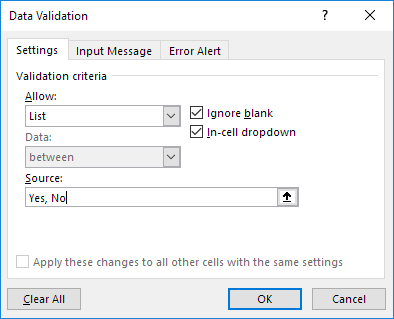
From the Settings tab you have to hit the Allow box, and then choose the List option.
Go to the Source box and choose the list range.

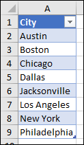
In the shown example we are putting our data on the sheet named as cities in the A2:A9.

Remember: we have left the header row just because we need not to include this in the selection area:

6. If you don’t want that empty cell to create any kind of issue then make a check across the Ignore blank Also tick the In-cell dropdown option.

7. Hit the Input Message

- To make a message box to pop-up when you make a tap over the cell, in that case you need to choose the “Show input message when cell is selected”
- Now assign the title and message which you want to show in the dialog box i.e. up to 255 characters.

In case, you don’t need to show any message then leave the option “show input message when cell is selected” unselected.

8. Go to the “Error Alert”.

In case to pop-up a message box when someone put anything wrong that is not present in your list, then make a check across the option “Show error alert after invalid data is entered” .

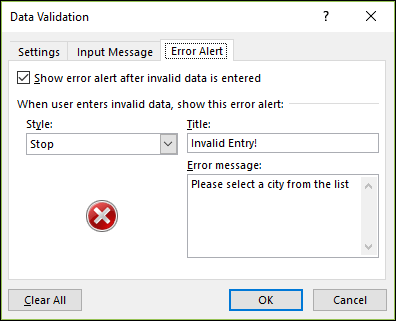
After that pick an option from the Style box: Information, Warning and stop. After that type the title and error message. If you don’t wants to display any pop-up message then remove the text from the error message section and uncheck the “show error alert after invalid data is entered”.

If you are confused about the options to choose from the Style box. Then read this out:

Information or warning: choosing this option will show the message but doesn’t prevent users from entering unavailable data of the drop-down list.

Stop: this option will stop users from inputting data which is not present in the drop-down list.

Note:

If you forgot to add the title or error message then by default the title will be considered as Microsoft Excel and message is taken as “The value you entered is not valid. A user has restricted values that can be entered into this cell.”

Method 2- Create Drop-Down List Using data From Cells

You can easily create drop-down list in Excel which allows other entries. Here are the steps that you need to perform:

Enter the value which is not available in the drop-down list after this Excel will display the error alert.

In this case, allow other entries, and perform the following steps.

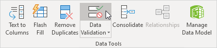
Go to the Data tab after that from Data Tools group, and hit the Data Validation icon.

This will open the dialog box of ‘Data Validation’.

Now you have to move onto the Error Alert tab and untick the ‘Show error alert after invalid data is entered’ option.
Hit the OK button.
Now you can very easily enter the value which is not present in the drop-down list.

Method 3- Dynamic Drop-Down List

Another very interesting way is to create dynamic drop–down list in Excel so that whenever any item is added or deleted from the list it automatically gets updated.

From your first sheet choose the cell B1.

Go to the Data tab and then from the Data Tools group hit the Data Validation icon.

This will automatically open the dialog box of ‘Data Validation’

From the Allow box, hit the List option.

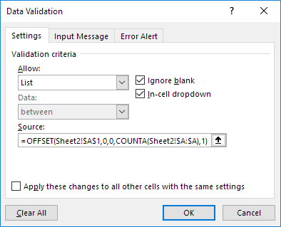
Tap on the Source box and after that enter this formula: =OFFSET(Sheet2!$A$1,0,0,COUNTA(Sheet2!$A:$A),1)

Explanation: here the Excel OFFSET function uses the 5 arguments. Reference: Sheet2!$A$1, rows to offset: 0, columns to offset: 0, height: COUNTA(Sheet2!$A:$A) and width: 1. COUNTA(Sheet2!$A:$A) counts the number of values in column A on Sheet2 that are not empty. When you add an item to the list on Sheet2, COUNTA(Sheet2!$A:$A) increases.

This will give you the result that range returned from the OFFSET function gets expanded and it will update the drop-down list also.

Hit the OK button.
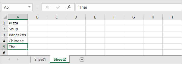
Go to the second sheet, and then add any new item at the list end.

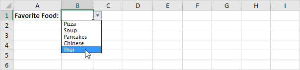
Result:

Method 4- Dependent Drop-down Lists

Let’s know how you can create a dependent drop-down list in Excel. Here is an example to show you how to create dependent drop-down lists in Excel.

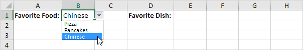
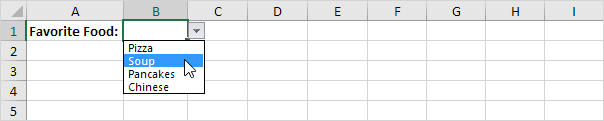
From one drop down list when the user chooses the pizza.

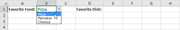
Then in the second drop-down list variants of pizza starts appearing. Perform the following steps to create dependent drop-down lists in Excel.

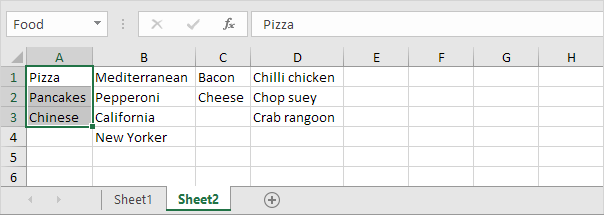
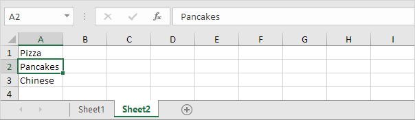
Go to the second sheet, for creating up the following named ranges.

Name	Range Address
Food	A1:A3
Pizza	B1:B4
Pancakes	C1:C2
Chinese	D1:D3

From your first sheet just choose the cell B1.

Go to the Data tab and after that from the Data Tools group, hit the Data Validation icon.

This will open the dialog box of ‘Data Validation’.

Now on the setting tab go to the Allow box make tap over the List option
In the Source box enter the text type =Food.

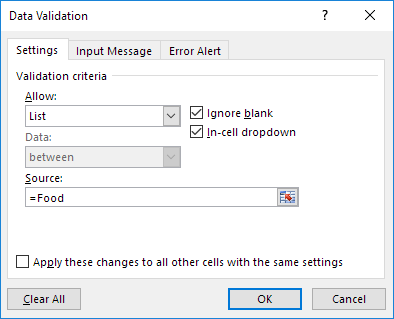
Hit the OK button.

Result:

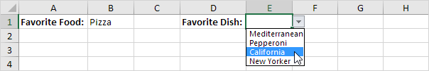
Now choose the cell E1.
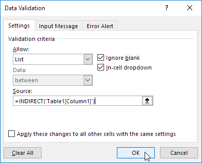
From the opened data validation dialog box go to the settings tab and then from the Allow box make tap over the List option.
In the Source box enter the text type =INDIRECT($B$1).

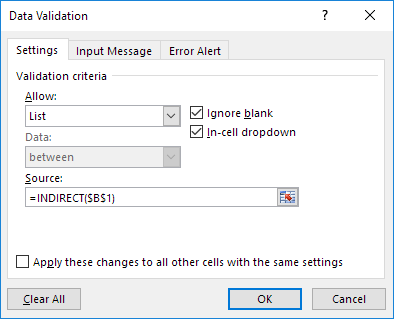
Press OK button.

Result:

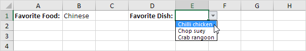
Explanation: here INDIRECT function will give you the reference mainly specified by the text string. Suppose if user selects the Chinese food category then from your first drop-down list. =INDIRECT($B$1). This will give you the Chinese item references. Due to this in the second drop-down list has the Chinese items.

Also Read: How to Insert/Create Calendar in Excel?

Method 5- How to Create Drop Down List in Excel Using Table Magic Method?

Another yet option that you can try for how to create drop-down list in Excel 2016 is Table Magic Method. This technique will help you for storing your items in MS Excel Table and even make a dynamic list.

Here is how you can use this method:

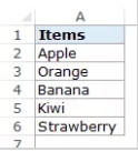
Select the list item in the sheet (as shown below).

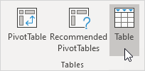
Next, click on ‘Insert Tab’ in tables group & choose ‘Table’

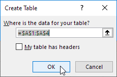
Now, Excel will select the stuff. Click on Ok.

In case, if you choose the list, Excel will display a structured reference
Now, you have to use a structured reference for creating a dynamic dropdown list.

After that, add a new entry at end of a list.
Finally, the table magic works & the new entry will be displayed on the drop-down list that you have added.

How to Add/Remove Items From Drop-Down List?

Even without using the ‘Data Validation’ option and making changes in the range reference, you can easily add/delete items from the drop-down list in Excel.

Let’s know how…!

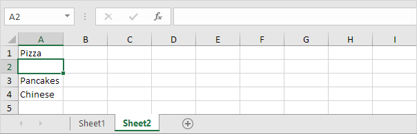
For adding an item in the drop-down list, choose the item first which you want to add.

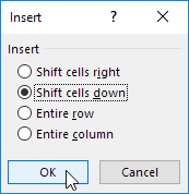
Make a right click, and hit the Insert option.

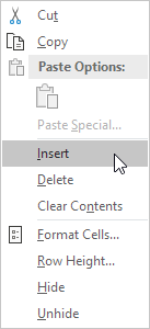
Choose the “Shift cells down” and hit the OK button.

Result:

Note:

You will notice that automatically the range reference is get shifted from Sheet2!$A$1:$A$3 to Sheet2!$A$1:$A$4. For checking this out, open the dialog box of ‘Data Validation’.

Enter any new item that you want to add.

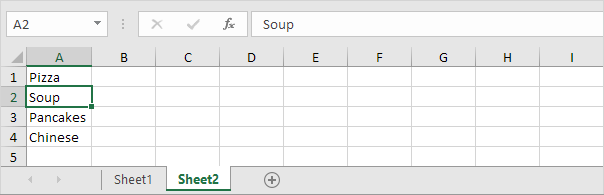
Here is the Result:

For removing any item from the drop-down list, got o step 2 and hit the Delete option. Choose the “Shift cells up” option and hit the OK tab.

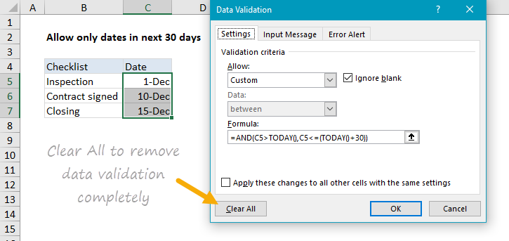
How to Remove A Drop-Down List in Excel?

Here are the steps that you need to perform for removing drop-down list in Excel.

Choose the cell having the drop-down list.
Go to the Data tab and then from the Data Tools group choose the Data Validation icon.

After this, you will see that a dialog box of ‘Data Validation’ starts appearing on your screen.

Hit the Clear All button.

Note:

For removing entire drop-down lists: on the opened data validation dialog box check the “Apply these changes to all other cells with the same settings” option right before selecting the Clear All button.

Hit the OK button.

How to Recover Corrupt/Lost/Deleted Excel File Data?

Have you ever thought about what initiative you will take if all of a sudden your Excel file data is lost or gets deleted somehow? Well, to deal with such a situation I have a simple solution i.e. to use Excel Recovery Tool, This software helps you to recover deleted, corrupted, lost Excel files even without any backup. Not only this it is also capable to repair corrupt, damaged Excel (XLS and XLSX) files and fix Excel errors as well.

With this, you can recover charts, chart sheets, tables, cell comments, images, cell comments, formulas, and sort & filter and all data components from corrupt Excel files.

Quickly recover and repair both .xls and .xlsx files.
Easily restore multiple corrupted Excel files simultaneously.
Restore everything including worksheets, cell comments, worksheet properties, charts, and other data.
Too easy to use so that even a novice user can also use it.
Supports both Windows as well as Mac operating systems.

Try Now Buy Now

* Free version of the product only previews recoverable data.

Final Verdict

So, this is all about how to create drop down list in Excel. Here, I have mentioned both the simple and dynamic ways to create Excel drop down list.

Besides, it is advised to handle your Excel file properly & create a valid backup of your data saved within it to avoid data loss circumstances.

Thanks for reading!

Priyanka Sahu

Priyanka is a content marketing expert. She writes tech blogs and has expertise in MS Office, Excel, and other tech subjects. Her distinctive art of presenting tech information in the easy-to-understand language is very impressive. When not writing, she loves unplanned travels.