A calendar in Microsoft Excel comes in handy if you’ve a busy schedule. Although an Excel calendar is an outstanding tool that can assist you to stay prepared when it comes to vital events, appointments, activities, meetings, etc. Therefore, today we are here to discuss how to create calendar in Excel or how to insert calendar in Excel effortlessly.
So, without any further ado, let’s get started…
To repair corrupt Excel file, we recommend this tool:
This software will prevent Excel workbook data such as BI data, financial reports & other analytical information from corruption and data loss. With this software you can rebuild corrupt Excel files and restore every single visual representation & dataset to its original, intact state in 3 easy steps:
- Try Excel File Repair Tool rated Excellent by Softpedia, Softonic & CNET.
- Select the corrupt Excel file (XLS, XLSX) & click Repair to initiate the repair process.
- Preview the repaired files and click Save File to save the files at desired location.
How To Create Calendar In Excel?
If you want to keep your data in a more organized way then a proper calendar system is very important for the right time management. Luckily Excel offers different ways to create calendars. Let’s know about each of them one by one in detail.
Method 1: Insert Calendar In Excel Using Date Picker Control
Well putting the drop-down calendar in Excel is quite easy to do but just because the time and date picker control are hidden so many users don’t know where it actually exists.
Here is the complete method to create a calendar in Excel perform this task step by step:
Note: Date Picker control of Microsoft works Microsoft’s very smoothly in the Excel 32-bit versions but not in Excel 64-bit version.
- Enable The Developer Tab on Excel ribbon.
Excel date picker control actually belongs to the ActiveX controls family, which comes under the Developer tab. Though this Excel Developer tab is kept hidden you can enable its visibility.
- On the Excel ribbon, you have to make a right-click, and after that choose the option Customize the Ribbon…. This will open the Excel options.
- From the opened window go to the right-hand side section. Now from customizing the ribbon section, you have to select the Main Tabs. In the appearing main tab list check the Developer box option and then click the OK button.

Also Read: How to Create a Flowchart in Excel? (Step-By-Step Guide)
- Insert The Calendar Control
Well, the Excel drop-down calendar is technically known as Microsoft Date and Time Picker Control.
To apply this in the Excel sheet, perform the following steps:
- Hit the Developer tab and then from the Controls group, you have to make a tap over arrow sign present within the Insert tab.
Now from the ActiveX Controls choose the “More Controls” button.

- From the opened dialog box of More Controlsselect the Microsoft Date and Time Picker Control 6.0 (SP6). After that click to the OK

- Hit the cell, in which you have to enter the calendar control.
You will see that a drop-down calendar control starts appearing on your Excel sheet:

Once this date picker control is been inserted, you will see that the EMBED formula starts appearing within the formula bar.
This gives detail to your Excel application about what kind of control is embedded within the sheet. You can’t change edit or delete this control because this will show the error “Reference is not valid“.
Adding the ActiveX control such date picker automatically enables the design mode which will allow you to change the properties and appearance of any freshly added control. The most obvious modification that you need to make at this time is resizing the calendar control and then linking it back to any specific cell.
For activating the Excel drop-down calendar option, hit the Design tab, and then from the Controls group, disable the Design Mode:
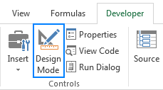
- Now, make a tap over the drop-down arrow for showing up the calendar and then select the date as per your need.
- Click the dropdown arrow to show the calendar in Excel and choose your desired date.

Note:
If MS date picker control is now not available within the list of More Controls. This situation mainly arises due to the following reasons.
- While you are running the MS Office 64 bit version. As there is no official date picker control available in the Office 64-bit.
- Calendar control i.e mscomct2.ocx is now not present or it is not registered on your PC.
- Customize Calendar Control
After the addition of the calendar control on your Excel sheet, now you have to shift this calendar control on the desired location and then resize it to get an easy fit within a cell.
- For resizing this date picker control, you have to enable the Design Mode after that drag this control from the corner section:

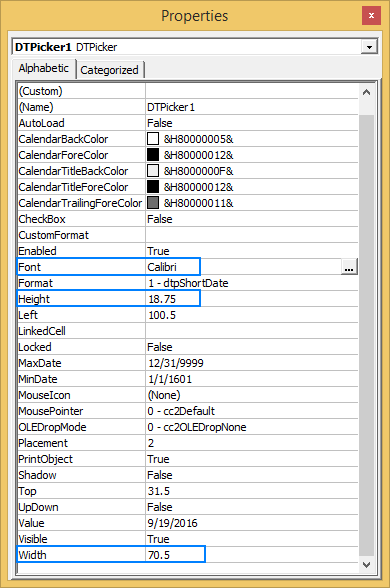
Or else you after enabling the Design Mode on, from the calendar control group choose the Properties tab:

- From the opened Properties window, you have to set the desired width, height, font size and style:
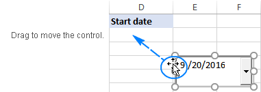
- To shift the Excel date picker control, place your mouse pointer over that and when the cursor changes into a four-pointed arrow sign, just drag the object wherever you want to place it.
- Link Excel Calendar Control With The Cell
After successfully adding the calendar drop-down in excel, you need to link it with some specific cell. This step very compulsory to perform if you want to make use of any selected dates with the formulas.
Suppose you are writing the formula for counting up the order’s number between any specific dates. For stopping any other from entering wrong dates such as 2/30/2016 you have inserted a drop-down calendar within 2 cells.
The COUNTIF formula that you have applied for calculating a number of orders will return the value “0” even if the orders are present.

Well, the main reason can be that your Excel is unable to recognize the value present in the date picker control. This problem will persist until you link the control with some specific cell. Here is the step that you need to perform:
- Selecting the calendar control you have to enable the Design Mode.
- Go to the Developer tab and then from the control group tap to the
- In the opened “Properties” windows, assign cell reference in the LinkedCell property (here I have written A3):

If Excel shows the following error “Can’t set cell value to NULL…” then click the OK button to ignore this.
After selecting the date from the drop-down calendar, the date will immediately start appearing in the linked cell. Now excel won’t face any issue in understanding the dates and the formula referencing done in the linked cells will work smoothly.

If you don’t need to have extra dates then link the date picker control with the cells where they are present.
Also Read: 4 Ways To Create Drop-Down List In Excel
Method 2: Using Excel Calendar Template
In Excel, there are handy graphic options with the clipart, tables, drawing tools, charts, etc. Using these options one can easily create a monthly calender or weekly calendar with special occasion dates or photos.
So go with the Excel calendar template which is the fastest and easiest way to create calendar in Excel using worksheet data.
Here are the steps to create calendar from Excel spreadsheet data using the template.
- Click the File> New after that in the search box you have to type “calendar”.
- Excel will make search thousands of online templates and then shows you the selected calendar templates which are grouped into the following categories.
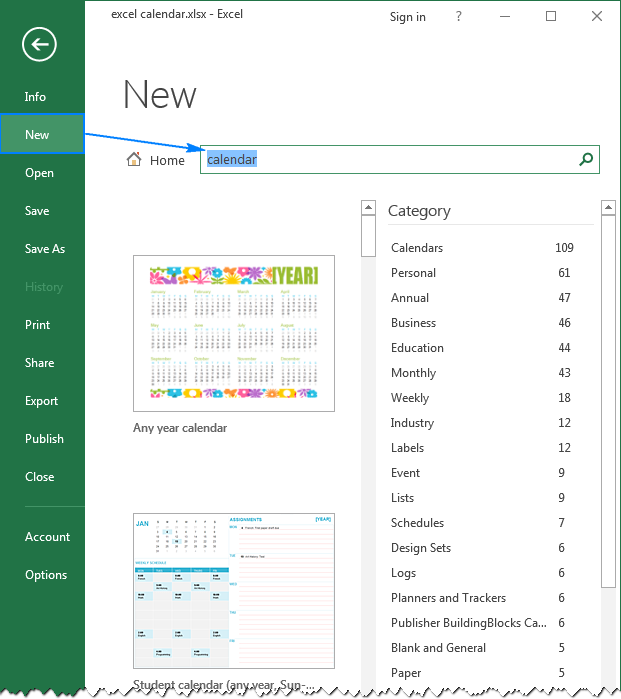
- Choose the calendar template as per your requirement, and then tap to the Create.

That’s all you need to do…!
Excel calendar template will be opened from the new Excel workbook and then print or customize as per your need. Usually, Excel weekly calendar templates are set with a year, whereas in some templates you can set a day for starting a week.
Note: for displaying always the current year in your excel calendar just assign a simple formula like this in the cell of the year: =YEAR(TODAY())

In this way, you can easily insert the drop-down calendar. Also, you can make a printable Excel calendar.
Method 3: Create Calendar In Excel Using VBA Code
In this method, you will get know-how using the Visual Basic for Applications(VBA) macro code you can create calendar in Excel.
- Open your Excel workbook.
- For excel 2003 users: Go to the Tools menu, and then hit the Macro tab. After that choose the Visual Basic Editor.
For Excel 2007 or later users: go to the Developer tab from the Excel ribbon and choose Visual Basic.
- From the Insert menu, choose the Module option.
- Now paste the VBA code which is given below into the opened sheet of the module.
- Go to the File menu and choose the Close and Return to Microsoft Excel.
- Now make a selection of the Sheet1
- From the Tools menu, go to the Macro tab. After that choose the Macros icon.
- Now you have to choose the CalendarMaker Now press the Run button to create Excel calendar.
Visual Basic Procedure To Create a Calendar In Excel:
You have to paste this code in the module sheet.
Sub CalendarMaker()
‘ Unprotect sheet if had previous calendar to prevent error.
ActiveSheet.Protect DrawingObjects:=False, Contents:=False, _
Scenarios:=False
‘ Prevent screen flashing while drawing calendar.
Application.ScreenUpdating = False
‘ Set up error trapping.
On Error GoTo MyErrorTrap
‘ Clear area a1:g14 including any previous calendar.
Range(“a1:g14”).Clear
‘ Use InputBox to get desired month and year and set variable
‘ MyInput.
MyInput = InputBox(“Type in Month and year for Calendar “)
‘ Allow user to end macro with Cancel in InputBox.
If MyInput = “” Then Exit Sub
‘ Get the date value of the beginning of inputted month.
StartDay = DateValue(MyInput)
‘ Check if valid date but not the first of the month
‘ — if so, reset StartDay to first day of month.
If Day(StartDay) <> 1 Then
StartDay = DateValue(Month(StartDay) & “/1/” & _
Year(StartDay))
End If
‘ Prepare cell for Month and Year as fully spelled out.
Range(“a1”).NumberFormat = “mmmm yyyy”
‘ Center the Month and Year label across a1:g1 with appropriate
‘ size, height and bolding.
With Range(“a1:g1”)
.HorizontalAlignment = xlCenterAcrossSelection
.VerticalAlignment = xlCenter
.Font.Size = 18
.Font.Bold = True
.RowHeight = 35
End With
‘ Prepare a2:g2 for day of week labels with centering, size,
‘ height and bolding.
With Range(“a2:g2”)
.ColumnWidth = 11
.VerticalAlignment = xlCenter
.HorizontalAlignment = xlCenter
.VerticalAlignment = xlCenter
.Orientation = xlHorizontal
.Font.Size = 12
.Font.Bold = True
.RowHeight = 20
End With
‘ Put days of week in a2:g2.
Range(“a2”) = “Sunday”
Range(“b2”) = “Monday”
Range(“c2”) = “Tuesday”
Range(“d2”) = “Wednesday”
Range(“e2”) = “Thursday”
Range(“f2”) = “Friday”
Range(“g2”) = “Saturday”
‘ Prepare a3:g7 for dates with left/top alignment, size, height
‘ and bolding.
With Range(“a3:g8”)
.HorizontalAlignment = xlRight
.VerticalAlignment = xlTop
.Font.Size = 18
.Font.Bold = True
.RowHeight = 21
End With
‘ Put inputted month and year fully spelling out into “a1”.
Range(“a1”).Value = Application.Text(MyInput, “mmmm yyyy”)
‘ Set variable and get which day of the week the month starts.
DayofWeek = WeekDay(StartDay)
‘ Set variables to identify the year and month as separate
‘ variables.
CurYear = Year(StartDay)
CurMonth = Month(StartDay)
‘ Set variable and calculate the first day of the next month.
FinalDay = DateSerial(CurYear, CurMonth + 1, 1)
‘ Place a “1” in cell position of the first day of the chosen
‘ month based on DayofWeek.
Select Case DayofWeek
Case 1
Range(“a3”).Value = 1
Case 2
Range(“b3”).Value = 1
Case 3
Range(“c3”).Value = 1
Case 4
Range(“d3”).Value = 1
Case 5
Range(“e3”).Value = 1
Case 6
Range(“f3”).Value = 1
Case 7
Range(“g3”).Value = 1
End Select
‘ Loop through range a3:g8 incrementing each cell after the “1”
‘ cell.
For Each cell In Range(“a3:g8”)
RowCell = cell.Row
ColCell = cell.Column
‘ Do if “1” is in first column.
If cell.Column = 1 And cell.Row = 3 Then
‘ Do if current cell is not in 1st column.
ElseIf cell.Column <> 1 Then
If cell.Offset(0, -1).Value >= 1 Then
cell.Value = cell.Offset(0, -1).Value + 1
‘ Stop when the last day of the month has been
‘ entered.
If cell.Value > (FinalDay – StartDay) Then
cell.Value = “”
‘ Exit loop when calendar has correct number of
‘ days shown.
Exit For
End If
End If
‘ Do only if current cell is not in Row 3 and is in Column 1.
ElseIf cell.Row > 3 And cell.Column = 1 Then
cell.Value = cell.Offset(-1, 6).Value + 1
‘ Stop when the last day of the month has been entered.
If cell.Value > (FinalDay – StartDay) Then
cell.Value = “”
‘ Exit loop when calendar has correct number of days
‘ shown.
Exit For
End If
End If
Next
‘ Create Entry cells, format them centered, wrap text, and border
‘ around days.
For x = 0 To 5
Range(“A4”).Offset(x * 2, 0).EntireRow.Insert
With Range(“A4:G4”).Offset(x * 2, 0)
.RowHeight = 65
.HorizontalAlignment = xlCenter
.VerticalAlignment = xlTop
.WrapText = True
.Font.Size = 10
.Font.Bold = False
‘ Unlock these cells to be able to enter text later after
‘ sheet is protected.
.Locked = False
End With
‘ Put border around the block of dates.
With Range(“A3”).Offset(x * 2, 0).Resize(2, _
7).Borders(xlLeft)
.Weight = xlThick
.ColorIndex = xlAutomatic
End With
With Range(“A3”).Offset(x * 2, 0).Resize(2, _
7).Borders(xlRight)
.Weight = xlThick
.ColorIndex = xlAutomatic
End With
Range(“A3”).Offset(x * 2, 0).Resize(2, 7).BorderAround _
Weight:=xlThick, ColorIndex:=xlAutomatic
Next
If Range(“A13”).Value = “” Then Range(“A13”).Offset(0, 0) _
.Resize(2, 8).EntireRow.Delete
‘ Turn off gridlines.
ActiveWindow.DisplayGridlines = False
‘ Protect sheet to prevent overwriting the dates.
ActiveSheet.Protect DrawingObjects:=True, Contents:=True, _
Scenarios:=True
‘ Resize window to show all of calendar (may have to be adjusted
‘ for video configuration).
ActiveWindow.WindowState = xlMaximized
ActiveWindow.ScrollRow = 1
‘ Allow screen to redraw with calendar showing.
Application.ScreenUpdating = True
‘ Prevent going to error trap unless error found by exiting Sub
‘ here.
Exit Sub
‘ Error causes msgbox to indicate the problem, provides new input box,
‘ and resumes at the line that caused the error.
MyErrorTrap:
MsgBox “You may not have entered your Month and Year correctly.” _
& Chr(13) & “Spell the Month correctly” _
& ” (or use 3 letter abbreviation)” _
& Chr(13) & “and 4 digits for the Year”
MyInput = InputBox(“Type in Month and year for Calendar”)
If MyInput = “” Then Exit Sub
Resume
End Sub
Note: You can customize the above code as per your requirement.
How Do I Make Excel Calendar Update Automatically?
Automatization is the chief strength of Microsoft Excel. However, if you need to create your calendar update automatically then use the formula mentioned below:
“= EOMONTH (TODAY() , – 1) +1”.
Well, the above formula employs “TODAY” feature to locate the present date & calculates the 1st day of the month with the “EOMONTH” feature.
Related FAQs:
Does Excel Have a Calendar Template?
Yes, of course, Microsoft Excel have a wide variety of calendar templates that can be used easily.
What Is the Formula to Create a Calendar in Excel?
=DATE(A2,A1,1) is the formula that can be used to create a calendar in MS Excel. All you need to do is to select the blank cell for showing the starting month’s date, then simply enter =DATE(A2,A1,1) in a formula bar >> press Enter key.
Can You Insert a Calendar into An Excel Cell?
YES, you can insert a calendar into an Excel cell. For this, you have to go to File menu >> select Close & Return to MS Excel. After this, select a tab ‘Sheet1’. On Tools menu, simply point to the Macro, & select Macros. choose CalendarMaker >> select the Run to create a calendar.
Wrap Up:
MS Excel offers its user a broad range of tools which will increase their productivity by using the projects, dates, and tracking events. In order to view the data of your Excel worksheet in calendar format, Microsoft will change your data and then import it into the Outlook. This will automatically change it into a calendar format.
Hopefully, you must have found an ample amount of information in this post. Thanks for reading this post….!

Priyanka Sahu
Priyanka is a content marketing expert. She writes tech blogs and has expertise in MS Office, Excel, and other tech subjects. Her distinctive art of presenting tech information in the easy-to-understand language is very impressive. When not writing, she loves unplanned travels.