Merging rows and columns in Microsoft Excel can improve your spreadsheet’s appearance & readability. Whether you’re designing a report or formatting a table, knowing how to merge cells efficiently is essential. In this helpful guide, you will learn how to merge rows and columns in Excel with ease.
To recover Excel data without any data loss, we recommend this tool:
This software will prevent Excel workbook data such as BI data, financial reports & other analytical information from corruption and data loss. With this software you can rebuild corrupt Excel files and restore every single visual representation & dataset to its original, intact state in 3 easy steps:
- Try Excel File Repair Tool rated Excellent by Softpedia, Softonic & CNET.
- Select the corrupt Excel file (XLS, XLSX) & click Repair to initiate the repair process.
- Preview the repaired files and click Save File to save the files at desired location.
How To Merge Rows And Columns In Excel Without Losing Data?
There are different methods for combining row and columns text in Excel. Here, check the ways one by one to merge data without losing it. First, check how to merge rows in Excel.
Part 1# How to Merge Rows in Excel
When it comes to merging the Excel rows there are two ways that allow you to merge rows data easily.
- Merge Excel rows using a formula
- Combine multiple rows using the Merge Cells add-in
1. How to Merge Multiple Rows using Excel Formulas
Excel provides various formulas that help you combine data from different rows. Possibly the easiest one is the CONCATENATE function. So here checks out some examples for concatenating numerous rows into one:
- Merge rows with spaces between data: For example =CONCATENATE(B1,” “,B2,” “,B3)
- Combine rows without any space between the values: For example =CONCATENATE(A1,A2,A3)
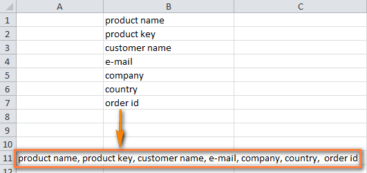
- Merge rows > separate the values with comma: For Example =CONCATENATE(A1,”, “,A2,”, “,A3)
Now check how the CONCATENATE formula works on the real data.

- On the sheet choose an empty cell and type the formula into it. Type the formula as per the data rows
- And copy the formula across entire other cells in the row.

- Now, simply you are having several data rows merged into one row.
2. How to Combine Rows in Excel using the Merge Cells Add-in

The Merge Cells add-in is used for merging various types of cells in Excel. This allows you to merges the individual cells and also combines data from entire rows or columns.
Please Note: You need to download a merge cell add-ins for third-party sites available online. Search in Google for add-ins.
Follow the given steps to combine two or more rows in your table:
- Choose rows you are looking to merge > click on the Merge Cells icon.
- Now the merge cells dialog window opens with a table or range selected already. And in the upper part of the window, you can see the three basic things:

-
- How you want to join cells – For combining rows of data > choose “column by column“.
- How to separate merged values with – an array of standard separators is available to choose from > comma, space, semicolon, and a line break. So select the separator as per your desire.
- Where you need to place the merged cells > either the top cell or the bottom cell?
- Now, check the lower part of the Windows to check if you need any additional options:

-
- Clear the content of selected cells – Choose this if need data to remain in the merged cells only.
- Merge all areas in the selection – This option allows you to merge rows in two or more non-adjacent ranges.
- Skip empty cells and Wrap text – Well, these are self-explanatory.
- Lastly, Create a backup copy of the worksheet – This option is checked by default. It is just a precaution that keeps you on the safe side and prevents the risk of data loss.
- Click the Merge button > to check the result – possible the merged rows of data separated by line breaks.
So, these are the two ways that allow you to merge rows in Excel without any data loss. Now, check out the ways on how to combine two columns in Excel.
Also Read: How to Remove Green Triangle in Excel? – Updated & Easy Guide!
Part 2# How to Merge Columns in Excel

Here, check out the 3 ways to merge data from several columns into one without using VBA macro.
- Merge two columns using formulas
- Combine columns data via NotePad
- The fastest way to join multiple columns
1. Merge Two Columns Using Excel Formulas
1. Into your table > insert a new column > in the column header, place the mouse pointer > right-click the mouse > select Insert from the context menu. Name the newly added columns for eg. – “Full Name”

2. In the cell D2, write the formula: =CONCATENATE(B2,” “,C2). The B2 and C2 are the addresses of First Name and Last Name. And in the formula, the quotation marks “” is the separator that will be inserted between merged names any other symbol can be used as a separator e.g. a comma.

3. Just like this, join data from several cells into one by making use of any separator of your choice.

4. Simply, copy the formula to other cells of the Full Name column. If the First name or the Last name is deleted, then the corresponding data in the Full name Column will also be gone.

5. Next, try converting the formula to a value so that you can remove the unnecessary columns from the Excel worksheet. Choose entire cells with data in the merged column (choose the first cell in “Full Name” Column > press Ctrl +Shift + Arrow Down)
6. Now copy the contents of the columns to clipboard > right click on the cell in the same column (“Full Name”) > choose “Paste Special” context menu > choose “Values” radio button > click OK.

7. Now remove “First Name” & “Last Name” columns that are not required. Click the column B header > press and hold Ctrl > click column C header.

8. After that make a right-click on any selected columns > select Delete from the context menu.
9. This is it, now you have successfully merged the names from 2 columns into one.

2. Combine columns Data via Notepad
This is another way that allows you to merge several columns. Here you don’t need any formulas. This is suitable for combining adjacent columns to make use of the same delimiter for all of them.
For Example: If looking for combining 2 columns with First Names and Last Names into one:
- Choose both columns you need to merge: Click B1 > press Shift + ArrrowRight for choosing C1 > then hit Ctrl + Shift + ArrowDown for choosing entire data cells with data in two columns.

- And copy data to clipboard > open Notepad > insert data from the clipboard to the Notepad

- Then copy tab character to clipboard > hit Tab right in Notepad > hit Ctrl + Shift + LeftArrow > press Ctrl + X.
- After that Replace Tab characters in Notepad with the separator, you require.
- Hit Ctrl + H for opening the “Replace” dialog box > paste the Tab character from the clipboard in Find what field > type the separator Space, comma etc in “Replace with” field. Hit the Replace All button > to close the dialog box press Cancel

- Now select the entire text in the Notepad and copy it to Clipboard.
- Then switch back to Excel worksheet (press Alt + Tab) > choose B1 cell and paste text from Clipboard to your table.

- And rename column B to “Full Name“ and remove the “Last name” column.
So, this is the second way that allows you to merge columns in Excel without any data loss.
3. Join Columns Using Merge Cells Add-in For Excel
This is the easiest and quickest way to combine data from numerous Excel columns into one. Just make use of the third party merge cells add-in for Excel.
And with the merge cells add-in, you can merge data from many cells by using any separator you like (for example carriage return or line break). With this, you can join row by row, column by column, or merge data from the selected cell into one without any loss.
There are many third-party add-ins sites online that allow you to download the add-ins and merge the cells easily in just a few clicks.
Frequently Asked Questions:
How to Merge Two Rows and Columns in an Existing Table?
You can combine two rows or columns in an existing table by following the below steps:
- Select the cell(s) to merge.
- On a table's Layout tab, choose Merge Cells in a Merge group.
When I Merge Cells, The Text Disappears in Excel.?
Many times, text disappears in Excel when merging cells and hinders in workflow. At the time, you have to right-click on a cell >> choose ‘Format Cells.’
Is There a Way to Merge Two Cells in Sheets and Keep All Data?
By using CONCATENATE formula, you can merge cells in sheets and keep all data in it. Excel provides various formulas and functions, CONCATENATE is one of them.
To merge two cells in Excel and keep the same data with a space, choose the cell you want to put a combined data. Then, type =CONCAT. Use commas to isolate the cells you’re combining, commas, use quotation marks to add spaces, other text, or the ampersand symbol (&) with the next cell that you want to combine.
Time to Sum Up
Merging cells in Excel helps format your spreadsheets more clearly. Whether you’re combining columns for a title or merging rows for better readability, follow the steps above to merge rows and columns in Excel effectively. For data safety, always back up before merging.
Keep your Excel sheets organized and professional with these easy tips!

Priyanka Sahu
Priyanka is a content marketing expert. She writes tech blogs and has expertise in MS Office, Excel, and other tech subjects. Her distinctive art of presenting tech information in the easy-to-understand language is very impressive. When not writing, she loves unplanned travels.