VLOOKUP (Vertical Lookup) is an excellent function that searches for an exact value in a first column of the table & returns a corresponding value from another column in a same row. But sometimes, you may face a situation where this function fails to work. In such a case, fixing this problem for a seamless spreadsheet experience is important. Well, this blog explores the most common reasons why VLOOKUP not working and how to fix it quickly.
To recover lost Excel data, we recommend this tool:
This software will prevent Excel workbook data such as BI data, financial reports & other analytical information from corruption and data loss. With this software you can rebuild corrupt Excel files and restore every single visual representation & dataset to its original, intact state in 3 easy steps:
- Try Excel File Repair Tool rated Excellent by Softpedia, Softonic & CNET.
- Select the corrupt Excel file (XLS, XLSX) & click Repair to initiate the repair process.
- Preview the repaired files and click Save File to save the files at desired location.
Why Is My VLOOKUP Not Working?
In this section, you will get an answer to this very important question why is VLookup not working. So, check out the 7 most common reasons for VLOOKUP not working in Excel 2007/2010/2013/2016/2019.
Have a look…
- VLOOKUP Can’t Find Value
- Table Reference Is Locked
- Column Insertion
- Oversized Table
- VLOOKUP Cannot Look To Its Left
- Not Getting The Exact Match
- Excel Table Has Duplicate Values
Reason 1# VLOOKUP Can’t Find Value
Excel user who all are using VLOOKUP, MATCH, or HLOOKUP functions every now and then encountered some unexpected #N/A error.
Usually, this error encounters when anyone tries to match the Excel lookup value within the array. It’s a clear sign that your Excel function has been failed to fetch lookup value from the lookup array.
What will you do if you will see that the exact matching value is there in the lookup array but your excel application is unable to find that value?
Suppose: if in the shown Excel spreadsheet, lookup function is applied. You want to look up the value “1110004” of the cell to get a match with the value “1110004” present in cell E6.

In this case, if the Excel function fails to fetch the match or showing error #N/A error. The VLOOKUP function is a popular lookup and reference function of Excel. It will show a tricky and dreaded #N/A error message. It may happen because Excel is not considering the two values exactly the same.
Reason 2# Table Reference Is Locked
If you are using multiple VLOOKUPs in excel to catch different information about any particular record. or if in case you are willing to copy off your VLOOKUP to several of your cells then you have to check your table.
The below-shown image shows that the VLOOKUP entered over here is incorrect. The incorrect cell ranges are referenced for the lookup_value and table array.

Solution
The table which is used by VLOOKUP function actually searches for and gives information is called astable_array. This is required to get referenced completely in order to copy your VLOOKUP.
So, click on the references which are right inside the formula and after then press the F4 key on your keyboard to modify the reference from relative to absolute. So, enter the formula as=VLOOKUP($H$3,$B$3:$F$11,4,FALSE).
In this example, both the lookup_value and table_array references made were absolute. Basically, it may be the table_array that needs locking.
Also Read: Why Does End Mode Excel Not Working? – Get Fixes Here!
Reason 3# Column Insertion
The column index number or col_index_num is used by the VLOOKUP function in order to enter information to return a record.
Because this is entered as an index number, and it is not that durable. If a column is put down in the table, then vlookup is not working as this stops VLOOKUP from working. Here is the image is shown below for a scenario.

The whole content is in column 3, but after the insertion of the new column, it became column 4. However, the VLOOKUP has not automatically updated.
Solution 1
One solution you can try to save your worksheet so any other user can’t insert columns. If the user requires to do so, then it’s not a valid solution.
Solution 2
Another option is to insert the MATCH function within the col_index_num argument of VLOOKUP.
The MATCH function can be used to search for something or returning the required column number. This will; makes the col_index_num dynamic so that the inserted columns won’t affect the VLOOKUP.
The formula given below needs to be entered within this example to avoid the above-mentioned problem.
Reason 4# Oversized Table
When more rows get added to the table, VLookup requires to get updated. Below given image shows that VLookup doesn’t check complete table fruit items.
Solution
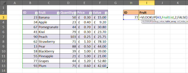
You can consider the formatting range as a dynamic range name or table (Excel 2007+). This process ensures that VLookup will look over the complete of your table.
In order to format the range as a table, choose the cell range that you want to use for table_array. After then tap to the Home > Format as Table and choose any one style from the gallery section. Tap to the Design tab present within Table Tools and then change the table name in the given box.
The VLOOKUP below shows a table named FruitList being used.
Reason 5# VLOOKUP Can’t Look On It’s Left
The limitation of the VLOOKUP function is that it can’t look at its left. This will appear at the left-most column of a table and return information from the right.
Solution
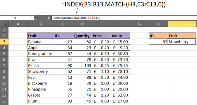
The solution to fix the VLOOKUP not working issue is not to use VLOOKUP at all. You can use the combination of INDEX and MATCH Excel function as an alternative for VLOOKUP.
The below given example is to show what information is returned to the left of the column you are looking in.
Reason 6# Not Getting The Exact Match
In the ending argument of VLOOKUP function, well known as range_lookup, you can search for the approximate or an exact match.
In most cases, users look for a particular product order, employee or customer and therefore require and an exact match. if you are searching for any unique value, enter FALSE for the range_lookup argument.
This one is optional, but if it is left unfilled then the TRUE value must be used. The TRUE value relies on your data is sorted in order to work.
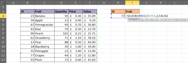
The Below shown figure will show a VLOOKUP with the range_lookup argument omitted and the incorrect value being returned.

Solution
If looking for some unique value then enter FALSE value for the ending argument. The VLOOKUP must be entered like =VLOOKUP(H3,B3: F11,2,FALSE).
This is the first reason behind the VLookup not working in Excel.
Reason 7# Excel Table Has Duplicate Values
Excel VLOOKUP function is limited to return only one record. It gives 1st record that matches the value you are searching for.
If your Excel table is having some duplicates then VLOOKUP fails to perform this task.
Solution
In the shown list some duplicates values are present. In this case, VLOOKUP is not the right choice to use. PivotTable is the perfect option to choose the value and then listing out the result.
Below shown table is to shows a list of orders. Suppose you are willing to return the entire order of any specific fruit.

PivotTable allows you to choose the Fruit ID from the report filter and the list of all orders starts appearing.

Automatic Solution: MS Excel Repair Tool
The given manual solution will surely fix your Excel file issues and errors. But if in case you are caught in any other corruption glitches or damaged file issues, then make use of the MS Excel Repair Tool. It is the best-suited software for restoring the corrupt Excel files and also for the retrieval of data from Excel worksheets like cell comments, charts, worksheet properties, and other stuff. It’s a professionally designed program that easily repairs .xls and .xlsx files.
Steps to Utilize MS Excel Repair Tool:


Best Practices to Avoid VLOOKUP Issues
Follow these precautionary measures to evade trouble in the future.
- Use exact match unless necessary.
- Always clean your data before applying formulas.
- Validate column index numbers regularly.
- Test your formulas with known values.
- Lock your table array with $ signs.
Related FAQs:
Why Does My VLOOKUP Show NA When Value Exists?
If your lookup column holds text values but your search query is formatted as numeric values, VLOOKUP show #N/A error.
How Do I Enable VLOOKUP In Excel?
To enable VLOOKUP in Excel, follow the below steps:
- Click the cell(s) where you need Excel to return a data you are looking for.
- Then, enter =VLOOKUP(lookup value,table array,column index number,range lookup).
- Lastly, press Enter.
What Is the Alternative To VLOOKUP?
XLOOKUP and INDEX/MATCH are the two recommended alternatives to VLOOKUP.
Why Isn't My VLOOKUP Working #Value?
VLOOKUP not working #value due to a typo in the col_index_num argument or unintentionally specifying a number less than 1 as the index value
How to Make VLOOKUP Work?
To make VLOOKUP function working again, follow the below steps.
- Select a cell ( H4 )
- Then, type =VLOOKUP.
- After that, double-click the VLOOKUP command.
- Select the cell(s) where search value will be entered ( H3 )
- Type ( , )
- Mark table range ( A2:E21 )
- Type ( , )
- Type the number of the column, counted from the left ( 2 ).
Final Verdict
VLOOKUP not working in Microsoft Excel is a frustrating issue, but solvable. However, by identifying the exact cause and applying the targeted fixes specified above, you can fix errors quickly. Clean your data, use exact match, and consider modern alternatives for better results.
Let your spreadsheets work smarter, not harder. I hope, you enjoyed reading this post.

Priyanka Sahu
Priyanka is a content marketing expert. She writes tech blogs and has expertise in MS Office, Excel, and other tech subjects. Her distinctive art of presenting tech information in the easy-to-understand language is very impressive. When not writing, she loves unplanned travels.