In MS Excel, errors like #DIV/0!, #N/A, and #VALUE! It often confuses readers. Well, the occurrence of such kinds of formula errors is a clear indication that you need to re-check the source. Whereas in most cases, such a formula error simply shows that the data used by the formulas is not present. However, it is important to remove errors in Excel to improve clarity and ensure your reports look professional. In this blog, you will learn how to hide errors in Excel in easy steps.
To fix corrupted Excel files, we recommend this tool:
This software will prevent Excel workbook data such as BI data, financial reports & other analytical information from corruption and data loss. With this software you can rebuild corrupt Excel files and restore every single visual representation & dataset to its original, intact state in 3 easy steps:
- Try Excel File Repair Tool rated Excellent by Softpedia, Softonic & CNET.
- Select the corrupt Excel file (XLS, XLSX) & click Repair to initiate the repair process.
- Preview the repaired files and click Save File to save the files at desired location.
How To Hide Errors In Excel?
The following are some easy tricks to hide errors in Excel.
- 1# Hide Error Values In A PivotTable Report
- 2# Hide Error Indicators In Cells
- 3#Hide Error Values By Turning The Text White
- 4# Hide Errors With The IFERROR Function
- 5# Hide All Error Values In Excel With Conditional Formatting
Trick 1# Hide Error Values In A PivotTable Report
- Make a tap over the PivotTable report it will start showing PivotTable Tools.
- Excel 2016/2013: Go to the Analyze tab and then to the PivotTable Now hit the arrow sign present next to the Options, after that choose the Options button.
Excel 2010/2007: From the Options tab>PivotTable group. Hit the arrow sign present next to Options, and after that choose the Options.

- Just hit the Layout & Format tab and try any of the following options:
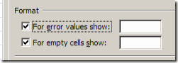
- Change Error Display: From the Format tab, choose the “For error values show”. In the appearing box, just assign the value which you want to show in place of errors.
In order to show errors like blank cells, just clear all the characters present in the box.
- Change Empty Cell Display:
From the Format tab choose the “For empty cells show” option. In the appearing box, just assign the value that you want to show in place of errors.
In order to show errors like blank cells, just clear all the characters present in the box. Whereas, to display zeros, just leave the check box empty.
Trick 2# Hide Error Indicators In Cells
If your cell is having a formula that is showing an error, then you will see a triangle, which is an error indicator. It appears in the cell’s top-left corner, and one can easily stop these indicators from appearing by trying the following steps:
- Select the formula cell that is having the problem
- In Excel 2016/ 2013/ 2010: Hit the File> Options >Formulas.
In Excel 2007: Hit the Microsoft Office Button > Excel Options > Formulas.
- In the opened Error Checking dialog box, just clear the check box of Enable background error checking.

Trick 3# Hide Error Values By Turning The Text White
By applying the white color to your text you can easily hide errors in Excel. This will make your text color completely invisible.
- Choose the cells range that has the error value.
- Go to the Home tab and in the Styles group, tap to the arrow sign present next to the Conditional Formatting.

- After that hit the Manage Rules option. This will open the dialog box of Conditional Formatting Rules Manager.
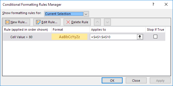
- Tap to the New Rule. After this, you will see a dialog box of New Formatting Rule will get open on your screen.
- From Select a Rule Type section hit the Format only cells that contain.
- Now, from the Format only cells with section go to the Edit the Rule Description option and hit the Errors.
- Go to the Format tab, and then make a tap over the Font.
- For opening up, the Color list hit the arrow sign and then from the Theme Colors choose the white color.

Trick 4# Hide Errors With The IFERROR Function
The easiest trick to hide error values in the Excel workbook is by using the IFERROR function. So by making use of the IFERROR function one can very easily replace the error that is appearing with another value or also with an alternative formula.
In the given example, the VLOOKUP function is showing the #N/A error value.
Well, the error has occurred because there is no Office detail assigned for searching. Not only this, it will start causing issues with the total calculation.
The IFERROR function efficiently handles the error value such as, #NAME!, #DIV/0!, #REF! Etc. this needs a value for checking up the error and if the error is encountered what task needs to perform.
In the above-given example, the VLOOKUP function is used for checking up the values, and instead of error “0” will be displayed.
Trick 5# Hide All Error Values In Excel With Conditional Formatting
Excel Conditional Formatting function can also help you in the task of hiding error values. Follow the below-given steps:
1. Choose the data range up to which you are willing to hide the formula errors.
2 Follow this path: Home > Conditional Formatting > New Rule.

3. Now from the opened dialog box of New Formatting Rule you have to select ”Use a formula to determine which cells to format” option which is present within the “Select a Rule Type”.
After that enter the formula: =ISERROR(A1) within the text box of “Format values where this formula is true”. (A1 is 1st cell that is present within the selected range which you can modify as per your need)

4. Hit the Format button this will open the Format Cells dialog box. After that select a white color for cell font from the Font.
Tips: Try to keep the font and background color the same. Suppose you have selected a red color for your background then choose red color also for the font.

5. To close the opened dialog box hit the OK You will see that entire error values will goes hidden at once.


Best Software For Recovering Missing Excel Workbook Data
If your Excel workbook data becomes corrupted, missing, or deleted, then you can make use of the MS Excel Repair Tool. This is the best tool to repair all sorts of issues, corruption, and errors in Excel workbooks. This tool allows you to easily restore all corrupt Excel file, including the charts, worksheet properties, cell comments, and other important data.
This is a unique tool to repair multiple Excel files at one repair cycle and recover the entire data in a preferred location. It is easy to use and compatible with both Windows as well as Mac operating systems. This software supports the entire Excel version.
Related FAQs:
How Do I Remove the Error Value in Excel?
You can remove the error value by copying all the cells & pasting only as values. In order to paste as only values, you have to select Home >> Paste option >> Paste Special >> Values. Doing this will eliminate all formulas & connections.
Where Is the Hide Function in Excel?
Navigate to Home tab, in the Cells group, then you have to click Format >> Visibility and then click on Hide & Unhide > Hide Sheet.
How Do I Hide #Value Error in Excel?
To hide this error, go to the File tab >> select Options and choose Formulas. In the Error Checking, clear the Enable background error checking check box.
Closure
Hiding errors in Microsoft Excel makes your worksheet cleaner and easier to read. Whether you use IFERROR, SUM, ISERROR, or conditional formatting, each method ensures your data stays professional. Nevertheless, by applying these practices, you can create sophisticated reports that impress colleagues and clients.
I hope this article seems informative to you. But if you have any more tricks to share, feel free to share them with us on our Facebook and Twitter pages.

Priyanka Sahu
Priyanka is a content marketing expert. She writes tech blogs and has expertise in MS Office, Excel, and other tech subjects. Her distinctive art of presenting tech information in the easy-to-understand language is very impressive. When not writing, she loves unplanned travels.