12 Ways To Clean Data In Excel Spreadsheet

Excel Spreadsheet is used by most of the users to store the data that they retrieve from different sources which may include unwanted data.

So to clean data in Excel spreadsheets becomes necessary as it will not only avoid and fix problems but also make the dataset look attractive and beautiful.

Cleaning data is a way of modifying information using different techniques. You can ensure that your data is usable, correct, and consistent.

Here in this blog, several methods are shown through which you can easily clean data in Excel spreadsheet.

Before knowing the techniques, let’s understand why cleaning of data in Excel is necessary.

Why Cleaning Data In Excel Spreadsheet Is Important?

Most of the users use multiple databases to import text files into Excel. This increases the high chances of getting data mislabeled or duplicated.

Industries like retail, banking, telecom, insurance, etc, rely on data for the growth of their business. It becomes important for these industries to keep their data error-free.

Removing data in Excel spreadsheets will help you to get rid of errors, inconsistency and also you can map different functions. Cleaning of data will increase marketing effectiveness.

In order to achieve maximum data efficiency, it is mandatory to remove all kinds of inconsistencies and data errors.

How To Remove Data In Excel Spreadsheet?

1: Clear Duplicate Data In Excel

You may have duplicate data all over Excel Spreadsheet and it may take time to find and remove those duplicates one by one.

So, here Excel helps you to clear it out within a short time. Go through the steps below to remove duplicate data:

• Firstly, click inside Excel Spreadsheet.
• Click on Table Tools.
• Click on Design.
• Then click on Remove Duplicate.

• Select the column that includes duplicate data and click OK.

2: Text To Column Feature

There may be the possibility of getting text cramped into a single cell while importing or exporting text files from or to the database.

In order to clean data in Excel Spreadsheet, you can parse the text into various cells using the text to column method.

• Select the text which you want to split into multiple cells.
• Click on the Data tab.
• In Data Tools, select Text to Columns.
• In Convert Text to Columns Wizard, select the Delimiters checkbox.

• Click on the Next button.
• Now, under Delimiter, only select the Space checkbox and leave the rest of the checkboxes.
• Click on the Finish button.

3: Convert Numbers

When you are importing or exporting text files from or to the database, then you may find numbers in text form which can cause issues, especially on calculation.

To avoid such issue further, follow the steps below:

• First, type 1 in any blank cell.
• Then where you have typed 1, select that cell and press Ctrl + C.
• Select the cells that you want to convert into numbers.
• Right-click and select Paste.
• Select Paste Special to open the Paste Special Dialogue box.
• In the operation section, select Multiply.

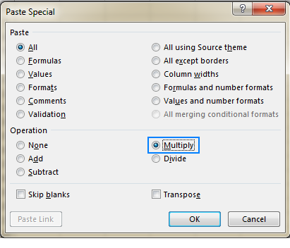
• Click Ok.

Now you will find your numbers back in numeric form.

4: Remove Blank Cells

Blank cells also may create further issues in your reports of Excel. If there is a small data set, then you can manually search and fill up those blank cells with 0 or Not Available.

In the case of a huge Excel file, you can select blank cells at a time using the below steps:

• Firstly, select the data set in Excel.
• To open Go To dialogue box, press F5.

• Now to open Go To Special dialogue box, select the Special…option.

• In Go To Special, select Blanks.
• Click on the OK button.

After applying these above steps, you will find all the blank cells in your data set. Now, you can fill up those blanks with 0 or not available, and after filling up press Ctrl + Enter.

5: Clean Inconsistency Data In Excel

Sometimes you may find text inconsistent while importing data from text files which makes your data set untidy.

You can use below mentioned some of the formulas to clean inconsistency data in Excel.

Formula 1. =REPLACE(A2,2,1,”o”)

Here, in this formula:

• A2 – position to replace
• 2 – where to start
• 1- number of characters to replace
• o – replace with

Example: Before Text: Sun    |     After Text: Son

Formula 2. =UPPER(A4)

Here, A4- Row number

Example: Before Text: will wallece  |     After Text: WILL WALLECE

Formula 3. =LOWER(A5)

Here, A5- Row number

Example: Before Text: Mary moore    |      After Text: mary moore

Formula 4. =PROPER(A6)

Here, A6- Row number

Example: Before Text: John jones       |      After Text: John Jones

Formula 5. =+SUBSTITUTE(A4,”-”,”/”)

Here, in this formula:

• A4 – Row number
• “-“: symbol to be replaced.
• “/”: symbol to be used in place of “-“

Example: Before Text: 267-483        |      After Text: 267/483

Formula 6. =CLEAN(A6)

Here, the A6-Row number.

Example: Before Text: Monthly$report |   After Text: Monthlyreport

Formula 7. =+TRIM(A5) (It allows to remove extra spaces)

Here, the A5-Row number.

Example: Before Text: 140 23        |      After Text: 14023

6: Find And Replace Feature

Excel has its inbuilt feature Find and Replace, which allows users to search for the particular data and replace it within seconds.

So, to replace data in Excel Spreadsheet, follow the below steps:

1. To open the Find and Replace dialogue box, press Ctrl + H.
2. Click on Replace.
3. In the Find what: box, enter data that you want to remove.
4. In Replace with box, enter data that you want to replace it.
5. You can replace particular data occurrences at a time by clicking on Replace All

7: Remove Formatting In Excel

To get data in excel, you might be using multiple databases. If you have all your data in one place then you can clear all formats.

Follow the below steps to remove formatting in excel:

1. Select your data set of Excel.
2. Click on the Home tab.
3. Select Clear.
4. Then select Clear Formats.

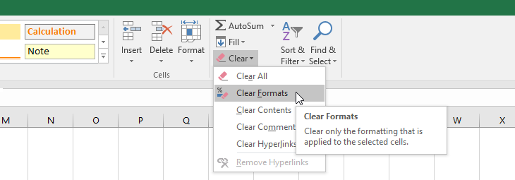
It will simply clean your all formatting in Excel. Using the above-given steps, you can also remove only hyperlinks, content, and comments.

8: Mark Errors In Data Set Of Excel

You can use Conditional formatting or the Go To Special technique to mark errors in the data set so that you can delete data or replace it with another data in Excel.

Follow the below steps for Conditional formatting:

• First, select the data set of Excel.
• Click on Home.
• Select Conditional Formatting.
• To open the New Formatting Rule dialogue box, select New Formatting Rule.

• Click on Format only cells that contain.
• In Edit the Rule Description:  select Errors under Format only cells with:
• Click on Format.
• Click Ok. This will mark the errors in your data set.

Now, here are the steps for Go To Special technique:

• Firstly, select the data set of Excel.
• To open Go To dialogue box, press F5.
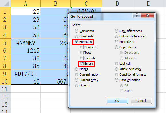
• Select Special located at the bottom left side.

• Select Formulas.
• Then select only Errors under Formulas and leave empty rest of the checkboxes.
• Click Ok. You can see errors marked up in your data set.

9: Delete Hidden Data In Excel

When you collect data from different sources, there may be hidden data such as names related to comments or documents author.

To avoid this hidden information, go through the below steps:

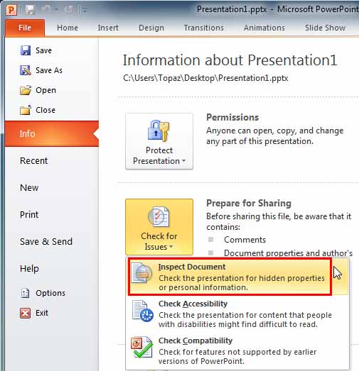
• First, click on File.
• Select Info.
• Select Check for Issues.
• Click on Inspect Document.

• Ensure that every checkbox is marked and then click on Inspect button.

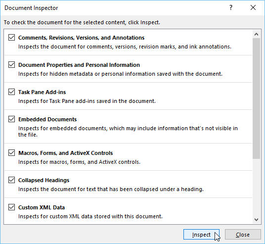
• Now click on Remove All button.

10: Check Spelling In  Excel

In order to keep data clean in Excel, it is important to keep checking spellings in Excel. It identifies the misspelled words and puts a red line below that misspelled or incorrect data.

To check the correctness of spellings, go through the steps below:

• First, select the range of the cell in Excel that you want to check spellings.
• Then just click on the F7 key on the keyboard.
• Now you will find the words that are misspelled in your selected data in Excel.

11: Fix Time And Date

There may be a possibility that time and date may get jumbled with hyphens or slash symbols of other strings. So, it is important to convert and reformat those jumbled data.

Use convert function to change time.

= CONVERT (number, from_unit, to_unit)    

number: row number where specific data is present and you want to convert it.

from_unit: give unit that you want to convert.

to_unit: give unit for further conversion.

Now to change time, go through the below steps:

• To change the hour value in time, enter this formula in Excel  = CONVERT (B2, “day”, “hr”) and hit Enter. It will show you the changed value in an hour with a calculation.
• To change the minute value in time, enter this formula in Excel = CONVERT (B2, “day”, “mn”) and hit Enter. It will produce the result.
• To change the second value in time, enter this formula in Excel = CONVERT (B2, “day”, “sec”) and hit Enter. It will give you the changed value.

You can convert your text date using the DATEVALUE function.

Now for the conversion of your text date, go through the below steps:

• Firstly, select the blank cell in Excel and check if its number format is in General or not.
• Now type DATEVALUE( in the blank cell.
• Select the date that is in the text format.
• Enter close bracket ).
• Then hit Enter and you will find the serial number of the text date.

• Now drag fill handle into blank cells range same as the range of text data cell.
• Select the serial number cell.
• In-Home tab, select Copy under Clipboard section.
• Select the text date cell.
• Again in the Home tab, click on the arrow below the Paste.
• Choose Paste Special.

• Now, select Values under Paste.
• Click Ok.
• In-Home tab, click on the corner arrow of the Number section to open the Number category.
• Click on Date under the Number category.
• Select the format of the date that you want from the Type list.

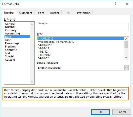
• Click on Ok. After the completion of the conversion, select the serial number cell and just press Delete.

12: Rotate Or Switch Cells

Sometimes while importing or exporting data in Excel, structured data in tabular format changes to unstructured data in nontabular format.

In order to transform data from columns to rows and rows to columns, use the =TRANSPOSE() function. Follow the below steps:

1. Select the blank cells as per cells of the original set. (In the below figure, you can see eight cells vertically which are the original set. So, here eight horizontal blank cells are selected.)

2. Type =TRANSPOSE() in the selected blank cells. (Verify that after typing the function, those eight cells are remaining selected.)

3. Now type the cell range in the function bracket that you want to transpose. (Same as shown in the figure)

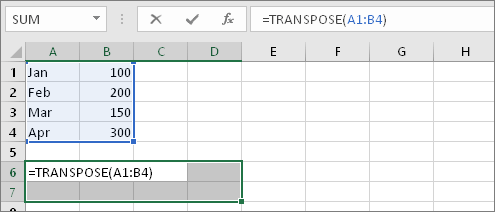
4. After typing, press CTRL + SHIFT + ENTER.

In this way, you can easily rearrange or transform columns and rows in your Excel.

Finishing Touch

Here, you have learned about different techniques that will help you to clean data in Excel spreadsheet.

Now, the problem arises when by mistake you remove data that you don’t want to. In this situation, you can use Excel Repair Tool to get back your images, charts, tables, formulas, cell comments, chart sheets, filters, and sorts of your data set.

Excel Repair Tool is capable of repairing multiple or single XLS/XLSX files. It can restore the worksheet with cell formatting and also can fix corruption errors in Excel.

In case, if you can’t access your Excel Spreadsheet due to some Excel errors or corruption then also you can use this tool.

The best thing about this tool is that it will not only restore the lost data but also you will find your restored data in original format and form.

Lastly, Excel Repair Tool supports every version of Excel and it is also available for Mac systems as well as Windows systems.